kaggle学习笔记
这部分的东西很碎,但是步骤是一样的,因此先记住大概的,然后一点一点的添东西就好
导入数据
import pandas as pd

# Read the test data
test = pd.read_csv('test.csv')
# Print train and test columns.查看列名(变量名)
print('Train columns:', train.columns.tolist())
print('Test columns:', test.columns.tolist())

# Read the sample submission file
sample_submission = pd.read_csv('sample_submission.csv')

# Look at the head() of the sample submission
print(sample_submission.head())
submission
Public vs Private leaderboard
这里的public和private没分太清呢
overfit
train :overfit:在训练集的误差大,而验证集的误差小,此时是训练集的过拟合
train_test_split
这个是划分训练集和测试集的
train_test_split函数可以将原始数据集按照一定比例划分训练集和测试集对模型进行训练
训练集和测试集的误差
要同时比较训练集和测试集的误差判断是否overfiting
from sklearn.metrics import mean_squared_error

dtrain = xgb.DMatrix(data=train[['store', 'item']])
dtest = xgb.DMatrix(data=test[['store', 'item']])

# For each of 3 trained models
for model in [xg_depth_2, xg_depth_8, xg_depth_15]:
    # Make predictions
    train_pred = model.predict(dtrain)
    test_pred = model.predict(dtest)

    # Calculate metrics
    mse_train =mean_squared_error(train['sales'], train_pred)
    mse_test = mean_squared_error(test['sales'], test_pred)
    print('MSE Train: {:.3f}. MSE Test: {:.3f}'.format(mse_train, mse_test))

<script.py> output:
    MSE Train: 631.275. MSE Test: 558.522
    MSE Train: 183.771. MSE Test: 337.337
    MSE Train: 134.984. MSE Test: 355.534
自定义误差函数
import numpy as np

# Import log_loss from sklearn
from sklearn.metrics import log_loss

# Define your own LogLoss function
def own_logloss(y_true, prob_pred):
  	# Find loss for each observation
    terms = y_true * np.log(prob_pred) + (1 - y_true) * np.log(1 - prob_pred)
    # Find mean over all observations
    err = np.mean(terms)
    return -err

print('Sklearn LogLoss: {:.5f}'.format(log_loss(y_classification_true, y_classification_pred)))
print('Your LogLoss: {:.5f}'.format(own_logloss(y_classification_true, y_classification_pred)))
EDA
PLOT
# Create hour feature
train['pickup_datetime'] = pd.to_datetime(train.pickup_datetime)
train['hour'] = train.pickup_datetime.dt.hour

# Find median fare_amount for each hour
hour_price = train.groupby('hour', as_index=False)['fare_amount'].median()

# Plot the line plot
plt.plot(hour_price['hour'], hour_price['fare_amount'], marker='o')
plt.xlabel('Hour of the day')
plt.ylabel('Median fare amount')
plt.title('Fare amount based on day time')
plt.xticks(range(24))
plt.show()
Local validation
Kfold
KFold交叉采样:将训练/测试数据集划分n_splits个互斥子集,每次只用其中一个子集当做测试集,剩下的(n_splits-1)作为训练集,进行n_splits次实验并得到n_splits个结果
# Import KFold
from sklearn.model_selection import KFold

# Create a KFold object
kf = KFold(n_splits=3, shuffle=True, random_state=123)

# Loop through each split
fold = 0
for train_index, test_index in kf.split(train):
    # Obtain training and testing folds
    cv_train, cv_test = train.iloc[train_index], train.iloc[test_index]
    print('Fold: {}'.format(fold))
    print('CV train shape: {}'.format(cv_train.shape))
    print('Medium interest listings in CV train: {}
'.format(sum(cv_train.interest_level == 'medium')))
    fold += 1

<script.py> output:
    Fold: 0
    CV train shape: (666, 9)
    Medium interest listings in CV train: 175

    Fold: 1
    CV train shape: (667, 9)
    Medium interest listings in CV train: 165

    Fold: 2
    CV train shape: (667, 9)
    Medium interest listings in CV train: 162
data leakage

划分时间特征
# Create TimeSeriesSplit object
time_kfold = TimeSeriesSplit(n_splits=3)

# Sort train data by date
train = train.sort_values('date')

# Iterate through each split
fold = 0
for train_index, test_index in time_kfold.split(train):
    cv_train, cv_test = train.iloc[train_index], train.iloc[test_index]

    print('Fold :', fold)
    print('Train date range: from {} to {}'.format(cv_train.date.min(), cv_train.date.max()))
    print('Test date range: from {} to {}
'.format(cv_test.date.min(), cv_test.date.max()))
    fold += 1

<script.py> output:
    Fold : 0
    Train date range: from 2017-12-01 to 2017-12-08
    Test date range: from 2017-12-08 to 2017-12-16

    Fold : 1
    Train date range: from 2017-12-01 to 2017-12-16
    Test date range: from 2017-12-16 to 2017-12-24

    Fold : 2
    Train date range: from 2017-12-01 to 2017-12-24
    Test date range: from 2017-12-24 to 2017-12-31
验证集的误差
from sklearn.model_selection import TimeSeriesSplit
import numpy as np

# Sort train data by date
train = train.sort_values('date')

# Initialize 3-fold time cross-validation
kf = TimeSeriesSplit(n_splits=3)

# Get MSE scores for each cross-validation split
mse_scores = get_fold_mse(train, kf)

print('Mean validation MSE: {:.5f}'.format(np.mean(mse_scores)))
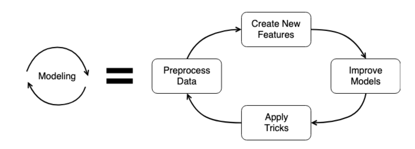
feature engineering
Arithmetical features
numerical
数值特征,可以直接做算数运算,进行拼接
# 这样做拼接的话是两个特征相加
train['TotalArea'] = train['TotalBsmtSF'] + train['FirstFlrSF'] + train['SecondFlrSF']
Date features
提取时间特征
pd.to_datetime
# Concatenate train and test together
taxi = pd.concat([train, test])

# Convert pickup date to datetime object
taxi['pickup_datetime'] = pd.to_datetime(taxi['pickup_datetime'])
# 提取星期
# Create a day of week feature
taxi['dayofweek'] = taxi['pickup_datetime'].dt.dayofweek

# 提取小时
# Create an hour feature
taxi['hour'] = taxi['pickup_datetime'].dt.hour

# Split back into train and test
new_train = taxi[taxi['id'].isin(train['id'])]
new_test = taxi[taxi['id'].isin(test['id'])]
Categorical features特征编码问题
是个大问题
label encoding
特征存在内在顺序 (ordinal feature)
one hot encoding
特征无内在顺序,category数量 < 4
target encoding (mean encoding, likelihood encoding, impact encoding)
特征无内在顺序,category数量 > 4
beta target encoding
特征无内在顺序,category数量 > 4, K-fold cross validation
不做处理(模型自动编码)
CatBoost,lightgbm
文本(分类)特征
有序的分类特征
无序的分类特征
处理方式有主要的两种,标签编码和独热编码
Label encoding
# Concatenate train and test together
houses = pd.concat([train, test])

# Label encoder
对于一个有m个category的特征,经过label encoding以后,每个category会映射到0到m-1之间的一个数。label encoding适用于ordinal feature (特征存在内在顺序)。
```r
#一般的实际案例是fit和transform分开的
from sklearn.preprocessing import LabelEncoder
le = LabelEncoder()

# Create new features
houses['RoofStyle_enc'] = le.fit_transform(houses['RoofStyle'])
houses['CentralAir_enc'] = le.fit_transform(houses['CentralAir'])

# Look at new features
print(houses[['RoofStyle', 'RoofStyle_enc', 'CentralAir', 'CentralAir_enc']].head())
<script.py> output:
      RoofStyle  RoofStyle_enc CentralAir  CentralAir_enc
    0     Gable              1          Y               1
    1     Gable              1          Y               1
    2     Gable              1          Y               1
    3     Gable              1          Y               1
    4     Gable              1          Y               1
one-hot
对于一个有m个category的特征,经过独热编码(OHE)处理后,会变为m个二元特征,每个特征对应于一个category。这m个二元特征互斥,每次只有一个激活。
独热编码解决了原始特征缺少内在顺序的问题,但是缺点是对于high-cardinality categorical feature (category数量很多),编码之后特征空间过大(此处可以考虑PCA降维),而且由于one-hot feature 比较unbalanced,树模型里每次的切分增益较小,树模型通常需要grow very deep才能得到不错的精度。因此OHE一般用于category数量 <4的情况。
# Concatenate train and test together
houses = pd.concat([train, test])

# Label encode binary 'CentralAir' feature
from sklearn.preprocessing import LabelEncoder
le = LabelEncoder()
houses['CentralAir_enc'] = le.fit_transform(houses['CentralAir'])

# Create One-Hot encoded features
ohe = pd.get_dummies(houses['RoofStyle'], prefix='RoofStyle')

# Concatenate OHE features to houses
houses = pd.concat([houses, ohe], axis=1)

# Look at OHE features
print(houses[[col for col in houses.columns if 'RoofStyle' in col]].head(3))
Target encoding
Mean target encoding
使用目标变量时,非常重要的一点是不要泄露任何验证集的信息。
所有基于目标编码的特征都应该在训练集上计算,接着仅仅合并或连接验证集和测试集。
即使验证集中有目标变量,它不能用于任何编码计算,否则会给出过于乐观的验证误差估计。
- Calculate the mean on the train, apply to the test
- Split train into K folds. Calculate the out-of-fold mean for each fold, apply to this particular fold
预测变量编码
def mean_target_encoding(train, test, target, categorical, alpha=5):

    # Get the train feature
    train_feature = train_mean_target_encoding(train, target, categorical, alpha)

    # Get the test feature
    test_feature = test_mean_target_encoding(train, test, target, categorical, alpha)

    # Return new features to add to the model
    return train_feature, test_feature
mean_target_encoding
这里理解的不太好。。。
k折交叉验证
# Create 5-fold cross-validation
kf = KFold(n_splits=5, random_state=123, shuffle=True)

# For each folds split
for train_index, test_index in kf.split(bryant_shots):
    cv_train, cv_test = bryant_shots.iloc[train_index], bryant_shots.iloc[test_index]

    # Create mean target encoded feature
    cv_train['game_id_enc'], cv_test['game_id_enc'] = mean_target_encoding(train=cv_train,
                                                                           test=cv_test,
                                                                           target='shot_made_flag',
                                                                           categorical='game_id',
                                                                           alpha=5)
    # Look at the encoding
    print(cv_train[['game_id', 'shot_made_flag', 'game_id_enc']].sample(n=1))
Missing data
处理缺失值
- xgboost和lightGBM不需要处理缺失值,因为可以自动处理
查看缺失值的数量
df.isnull().sum()
均值填充
# Import SimpleImputer
from sklearn.impute import SimpleImputer

# Create mean imputer
mean_imputer = SimpleImputer(strategy='mean')

# Price imputation
rental_listings[['price']] = mean_imputer.fit_transform(rental_listings[['price']])
Baseline model
这个我打算做一个实例,视频这部分有点糊,不过kaggle官网上面确实有很多有用的baseline,有些流程是固定的,可以有一个大体思路之后继续。