pandas包学习笔记

pandas

pandas

是基于numpy和matplotlib的

import pandas as pd

# Print the values of homelessness
print(homelessness.values)

# Print the column index of homelessness
print(homelessness.columns)

# Print the row index of homelessness
print(homelessness.index)

.values:查看每列的值
.columns：查看所有列名
.index：查看索引

zip

zip() 函数用于将可迭代对象作为参数，将对象中对应的元素打包成一个个元组，然后返回由这些元组组成的对象。
如果各个可迭代对象的元素个数不一致，则返回的对象长度与最短的可迭代对象相同。简书
利用 * 号操作符，与zip相反，进行解压。

# Zip the 2 lists together into one list of (key,value) tuples: zipped
zipped = list(zip(list_keys,list_values))

# Inspect the list using print()
print(zipped)

# Build a dictionary with the zipped list: data
data = dict(zipped)

# Build and inspect a DataFrame from the dictionary: df
df = pd.DataFrame(data)
print(df)

read_csv

# Read in the file: df1
df1 = pd.read_csv(data_file)

# Create a list of the new column labels: new_labels
new_labels = ['year', 'population']

# Read in the file, specifying the header and names parameters: df2
df2 = pd.read_csv(data_file, header=0, names=new_labels)

# Print both the DataFrames
print(df1)
print(df2)

与r相比，读入数据的时候不用加引号

# Read the raw file as-is: df1
df1 = pd.read_csv(file_messy)

# Print the output of df1.head()
print(df1.head())

# Read in the file with the correct parameters: df2
df2 = pd.read_csv(file_messy, delimiter=' ', header=3, comment='#')

# Print the output of df2.head()
print(df2.head())

# Save the cleaned up DataFrame to a CSV file without the index
df2.to_csv(file_clean, index=False)

# Save the cleaned up DataFrame to an excel file without the index
df2.to_excel('file_clean.xlsx', index=False)
<script.py> output:
                                                       The following stock data was collect on 2016-AUG-25 from an unknown source
    These kind of comments are not very useful                                                  are they?                        
    Probably should just throw this line away too          but not the next since those are column labels                        
    name Jan Feb Mar Apr May Jun Jul Aug Sep Oct No...                                                NaN                        
    # So that line you just read has all the column...                                                NaN                        
    IBM 156.08 160.01 159.81 165.22 172.25 167.15 1...                                                NaN                        
         name     Jan     Feb     Mar     Apr  ...     Aug     Sep     Oct     Nov     Dec
    0     IBM  156.08  160.01  159.81  165.22  ...  152.77  145.36  146.11  137.21  137.96
    1    MSFT   45.51   43.08   42.13   43.47  ...   45.51   43.56   48.70   53.88   55.40
    2  GOOGLE  512.42  537.99  559.72  540.50  ...  636.84  617.93  663.59  735.39  755.35
    3   APPLE  110.64  125.43  125.97  127.29  ...  113.39  112.80  113.36  118.16  111.73
    [4 rows x 13 columns]

Plotting with pandas

是基于matplotlib的
熊猫绘图，哈哈哈

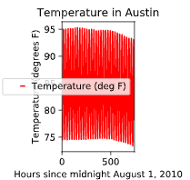
# Create a plot with color='red'设置线条颜色
df.plot(color='red')

# Add a title自定义标题

plt.title('Temperature in Austin')
# Specify the x-axis label 自定义x轴标题
plt.xlabel('Hours since midnight August 1, 2010')

# Specify the y-axis label 自定义y轴标题
plt.ylabel('Temperature (degrees F)')

# Display the plot 
plt.show()

不知道可否这样理解，于Python来讲，就是在调用方法？？

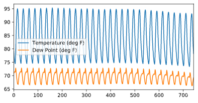
 Plot all columns (default)
df.plot()
plt.show()

# Plot all columns as subplots
df.plot(subplots=True)
plt.show()
# Plot just the Dew Point data
column_list1 = ['Dew Point (deg F)']
df[column_list1].plot()
plt.show()
# Plot the Dew Point and Temperature data, but not the Pressure data
column_list2 = ['Temperature (deg F)','Dew Point (deg F)']
df[column_list2].plot()
plt.show()

Visual exploratory data analysis

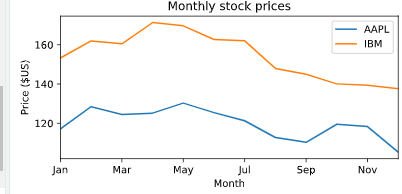
折线图

# Create a list of y-axis column names: y_columns
y_columns = ['AAPL', 'IBM']

# Generate a line plot
df.plot(x='Month', y=y_columns)

# Add the title
plt.title('Monthly stock prices')

# Add the y-axis label
plt.ylabel('Price ($US)')

# Display the plot
plt.show()

散点图

# Generate a scatter plot
df.plot(kind='scatter', x='hp', y='mpg',s=sizes)

# Add the title
plt.title('Fuel efficiency vs Horse-power')

# Add the x-axis label
plt.xlabel('Horse-power')

# Add the y-axis label
plt.ylabel('Fuel efficiency (mpg)')

# Display the plot
plt.show()

目前可以看出来学习R 包的套路和python包的套路是一致的

# Make a list of the column names to be plotted: cols
cols = ['weight' , 'mpg']

# Generate the box plots
df[cols].plot(kind='box',subplots=True)

# Display the plot
plt.show()

有包的可以掉包，不过应该是主要集中于一些基本的包，希望还是可以自己写一些包，或者函数。这样可以实现自己想实现的功能。

panadas hist pdf cdf

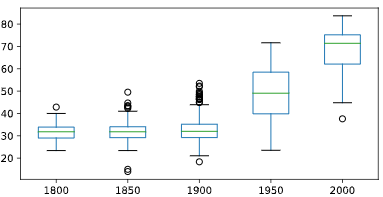
Statistical exploratory data analysis

# Print the number of countries reported in 2015
print(df['2015'].count())

# Print the 5th and 95th percentiles
print(df.quantile([0.05,0.95]))

# Generate a box plot
years = ['1800','1850','1900','1950','2000']
df[years].plot(kind='box')
plt.show()

其实有时候觉得，写这么多的代码应该是无用的，记一些常见的封装好的函数以后也会忘记的，真正的是解决问题的思路是要整明白的
慢慢来吧，代码量应该是不够的

descripe

这个函数就是R里面的summary函数，描述统计信息

Separating populations

常记的几个函数

describe
head
loc
iloc

index series

# Prepare a format string: time_format
time_format = '%Y-%m-%d %H:%M'

# Convert date_list into a datetime object: my_datetimes
my_datetimes = pd.to_datetime(date_list, format=time_format)  

# Construct a pandas Series using temperature_list and my_datetimes: time_series
time_series = pd.Series(temperature_list, index=my_datetimes)

resample()

重新确定frequency的函数，可以结合基础函数如：agg，groupby，mean等，进行时间序列批量处理
可以进行某一时间段的统计

# Downsample to 6 hour data and aggregate by mean: df1
df1 = df.loc[:,'Temperature'].resample('6h').mean()

# Downsample to daily data and count the number of data points: df2
df2 = df.loc[:,'Temperature'].resample('D').count()

date
2010-01-01 00:00:00    44.200000
2010-01-01 06:00:00    45.933333
2010-01-01 12:00:00    57.766667
2010-01-01 18:00:00    49.450000
2010-01-02 00:00:00    44.516667
Freq: 6H, Name: Temperature, dtype: float64
Date
2010-01-01    24
2010-01-02    24
2010-01-03    24
2010-01-04    24
2010-01-05    24
Freq: D, Name: Temperature, dtype: int64

比如这个demo

# Extract temperature data for August: august
august = df['Temperature']['2010-August']

# Downsample to obtain only the daily highest temperatures in August: august_highs
august_highs = august.resample('D').max()

# Extract temperature data for February: february
february = df['Temperature']['2010-Feb']

# Downsample to obtain the daily lowest temperatures in February: february_lows
february_lows = february.resample('D').min()

.str.contains()

查询待匹配的xx

# Extract data for which the destination airport is Dallas: dallas
dallas = df['Destination Airport'].str.contains('DAL')

# Reset the index of ts2 to ts1, and then use linear interpolation to fill in the NaNs: ts2_interp
ts2_interp = ts2.reindex(ts1.index).interpolate(how='linear')

# Compute the absolute difference of ts1 and ts2_interp: differences 
differences = np.abs(ts1 - ts2_interp)

# Generate and print summary statistics of the differences
print(differences.describe())

**reindex就是重新定义索引，这个函数挺好用的，并且重新定义索引的方法不仅仅这一个,可以多多积累

时区处理方法

# Combine two columns of data to create a datetime series: times_tz_none 
times_tz_none = pd.to_datetime( la['Date (MM/DD/YYYY)'] + ' ' + la['Wheels-off Time'] )

# Localize the time to US/Central: times_tz_central
times_tz_central = times_tz_none.dt.tz_localize('US/Central')

# Convert the datetimes from US/Central to US/Pacific转化为太平洋时区
times_tz_pacific = times_tz_central.dt.tz_convert('US/Pacific')

导入和处理数据

最基本的导入数据

# Import pandas
import pandas as pd

# Read in the data file: df
df = pd.read_csv(data_file)

# Print the output of df.head()
print(df.head())

# Read in the data file with header=None: df_headers
df_headers = pd.read_csv(data_file, header=None)

# Print the output of df_headers.head()
print(df_headers.head())

drop()

删除某行或者某列

突然发现pd.to_与R语言的as.的作用是一样的可以直接转化成某种类型

总结

感觉单独学这个视频的作用不大，和pandas 处理时间序列的视频课程基本上是重复的
还是多看看实际项目的应用吧，还有就是进pandas官网学习

numpy的笔记还没看。。先去学下