Tidyverse 学习笔记
1.gapminder 我理解的gapminder应该是一个内置的数据集
加载之后使用
> # Load the gapminder package
> library(gapminder)
> # Load the dplyr package
> library(dplyr)
> # Look at the gapminder dataset
> gapminder
A tibble: 1,704 x 6
   country     continent  year lifeExp      pop gdpPercap
   <fct>       <fct>     <int>   <dbl>    <int>     <dbl>
 1 Afghanistan Asia       1952    28.8  8425333      779.
 2 Afghanistan Asia       1957    30.3  9240934      821.
 3 Afghanistan Asia       1962    32.0 10267083      853.
 4 Afghanistan Asia       1967    34.0 11537966      836.
 5 Afghanistan Asia       1972    36.1 13079460      740.
 6 Afghanistan Asia       1977    38.4 14880372      786.
 7 Afghanistan Asia       1982    39.9 12881816      978.
 8 Afghanistan Asia       1987    40.8 13867957      852.
 9 Afghanistan Asia       1992    41.7 16317921      649.
10 Afghanistan Asia       1997    41.8 22227415      635.
 ... with 1,694 more rows
1.1 filter 函数
解释:过滤/筛选,按条件,可以有很多条件
gapminder %>%filter(year==2002,country=="China")
A tibble: 1 x 6
  country continent  year lifeExp        pop gdpPercap
  <fct>   <fct>     <int>   <dbl>      <int>     <dbl>
1 China   Asia       2002    72.0 1280400000     3119.
1.2 排序函数arrange,默认升序,参数desc降序
> # Sort in ascending order of lifeExp
> gapminder %>%
    arrange(lifeExp)
 A tibble: 1,704 x 6
   country      continent  year lifeExp     pop gdpPercap
   <fct>        <fct>     <int>   <dbl>   <int>     <dbl>
 1 Rwanda       Africa     1992    23.6 7290203      737.
 2 Afghanistan  Asia       1952    28.8 8425333      779.
 3 Gambia       Africa     1952    30    284320      485.
 4 Angola       Africa     1952    30.0 4232095     3521.
 5 Sierra Leone Africa     1952    30.3 2143249      880.
 6 Afghanistan  Asia       1957    30.3 9240934      821.
 7 Cambodia     Asia       1977    31.2 6978607      525.
 8 Mozambique   Africa     1952    31.3 6446316      469.
 9 Sierra Leone Africa     1957    31.6 2295678     1004.
10 Burkina Faso Africa     1952    32.0 4469979      543.
... with 1,694 more rows
按照lifeExp 降序
> # Sort in descending order of lifeExp
> gapminder %>%
    arrange(desc(lifeExp))
 A tibble: 1,704 x 6
   country          continent  year lifeExp       pop gdpPercap
   <fct>            <fct>     <int>   <dbl>     <int>     <dbl>
 1 Japan            Asia       2007    82.6 127467972    31656.
 2 Hong Kong, China Asia       2007    82.2   6980412    39725.
 3 Japan            Asia       2002    82   127065841    28605.
 4 Iceland          Europe     2007    81.8    301931    36181.
 5 Switzerland      Europe     2007    81.7   7554661    37506.
 6 Hong Kong, China Asia       2002    81.5   6762476    30209.
 7 Australia        Oceania    2007    81.2  20434176    34435.
 8 Spain            Europe     2007    80.9  40448191    28821.
 9 Sweden           Europe     2007    80.9   9031088    33860.
10 Israel           Asia       2007    80.7   6426679    25523.
 ... with 1,694 more rows
筛选和排序组合使用:
> library(gapminder)
> library(dplyr)
>
> # Filter for the year 1957, then arrange in descending order of population
> gapminder%>%filter(year==1957)%>%arrange(desc(pop))
A tibble: 142 x 6
   country        continent  year lifeExp       pop gdpPercap
   <fct>          <fct>     <int>   <dbl>     <int>     <dbl>
 1 China          Asia       1957    50.5 637408000      576.
 2 India          Asia       1957    40.2 409000000      590.
 3 United States  Americas   1957    69.5 171984000    14847.
 4 Japan          Asia       1957    65.5  91563009     4318.
 5 Indonesia      Asia       1957    39.9  90124000      859.
 6 Germany        Europe     1957    69.1  71019069    10188.
 7 Brazil         Americas   1957    53.3  65551171     2487.
 8 United Kingdom Europe     1957    70.4  51430000    11283.
 9 Bangladesh     Asia       1957    39.3  51365468      662.
10 Italy          Europe     1957    67.8  49182000     6249.
... with 132 more rows
2 mutute 函数
2.1 修改变量,并且将新变量增加到数据框或者矩阵的左侧
> # Use mutate to change lifeExp to be in months
> gapminder%>%mutate(lifeExp=12*lifeExp)
 A tibble: 1,704 x 6
   country     continent  year lifeExp      pop gdpPercap
   <fct>       <fct>     <int>   <dbl>    <int>     <dbl>
 1 Afghanistan Asia       1952    346.  8425333      779.
 2 Afghanistan Asia       1957    364.  9240934      821.
 3 Afghanistan Asia       1962    384. 10267083      853.
 4 Afghanistan Asia       1967    408. 11537966      836.
 5 Afghanistan Asia       1972    433. 13079460      740.
 6 Afghanistan Asia       1977    461. 14880372      786.
 7 Afghanistan Asia       1982    478. 12881816      978.
 8 Afghanistan Asia       1987    490. 13867957      852.
 9 Afghanistan Asia       1992    500. 16317921      649.
10 Afghanistan Asia       1997    501. 22227415      635.
... with 1,694 more rows
>
2.2 增加新的变量
>  Use mutate to create a new column called lifeExpMonths
> gapminder%>%mutate(lifeExpMonths=12*lifeExp)
 A tibble: 1,704 x 7
   country     continent  year lifeExp      pop gdpPercap lifeExpMonths
   <fct>       <fct>     <int>   <dbl>    <int>     <dbl>         <dbl>
 1 Afghanistan Asia       1952    28.8  8425333      779.          346.
 2 Afghanistan Asia       1957    30.3  9240934      821.          364.
 3 Afghanistan Asia       1962    32.0 10267083      853.          384.
 4 Afghanistan Asia       1967    34.0 11537966      836.          408.
 5 Afghanistan Asia       1972    36.1 13079460      740.          433.
 6 Afghanistan Asia       1977    38.4 14880372      786.          461.
 7 Afghanistan Asia       1982    39.9 12881816      978.          478.
 8 Afghanistan Asia       1987    40.8 13867957      852.          490.
 9 Afghanistan Asia       1992    41.7 16317921      649.          500.
10 Afghanistan Asia       1997    41.8 22227415      635.          501.
... with 1,694 more rows
2.3 combine
> library(gapminder)
> library(dplyr)
> # Filter, mutate, and arrange the gapminder dataset
> gapminder%>%filter(year==2007)%>%mutate(
  lifeExpMonths=12 * lifeExp,
  )%>%arrange(desc(lifeExpMonths))
 A tibble: 142 x 7
   country          continent  year lifeExp       pop gdpPercap lifeExpMonths
   <fct>            <fct>     <int>   <dbl>     <int>     <dbl>         <dbl>
 1 Japan            Asia       2007    82.6 127467972    31656.          991.
 2 Hong Kong, China Asia       2007    82.2   6980412    39725.          986.
 3 Iceland          Europe     2007    81.8    301931    36181.          981.
 4 Switzerland      Europe     2007    81.7   7554661    37506.          980.
 5 Australia        Oceania    2007    81.2  20434176    34435.          975.
 6 Spain            Europe     2007    80.9  40448191    28821.          971.
 7 Sweden           Europe     2007    80.9   9031088    33860.          971.
 8 Israel           Asia       2007    80.7   6426679    25523.          969.
 9 France           Europe     2007    80.7  61083916    30470.          968.
10 Canada           Americas   2007    80.7  33390141    36319.          968.
... with 132 more rows
3 浅谈:ggplot2 绘图
基本的制图,不添加任何图形元素是可以看下面的小demo,但是用到其他的元素了,就可以
https://cran.r-project.org/web/packages/ggplot2/ggplot2.pdf这个说明文当还是挺全面的
library(gapminder)
library(dplyr)
library(ggplot2)

gapminder_1952 <- gapminder %>%
  filter(year == 1952)

Change to put pop on the x-axis and gdpPercap on the y-axis
ggplot(gapminder_1952, aes(x = pop, y = gdpPercap)) +
  geom_point()

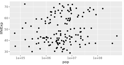
3.1 x坐标取对数
zheyang
> library(gapminder)
> library(dplyr)
> library(ggplot2)
>
> gapminder_1952 <- gapminder %>%
    filter(year == 1952)
>
> # Change this plot to put the x-axis on a log scale
> ggplot(gapminder_1952, aes(x = pop, y = lifeExp)) +
    geom_point()+
    scale_x_log10()
> library(gapminder)
> library(dplyr)
> library(ggplot2)
>
> gapminder_1952 <- gapminder %>%
    filter(year == 1952)
>
> # Change this plot to put the x-axis on a log scale
> ggplot(gapminder_1952, aes(x = pop, y = lifeExp)) +
    geom_point()+
    scale_x_log10()+
    scale_y_log10()
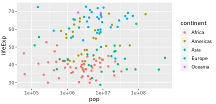
3.2 设置color和size
设置国家的颜色是不一样的
 gapminder_1952 <- gapminder %>%
    filter(year == 1952)
>
> # Scatter plot comparing pop and lifeExp, with color representing continent
> ggplot(gapminder_1952,aes(x=pop,y=lifeExp,colour= continent))+geom_point()+
  scale_x_log10()
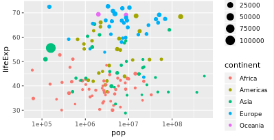
3.3 设置size
> gapminder_1952 <- gapminder %>%
    filter(year == 1952)
>
> # Add the size aesthetic to represent a country's gdpPercap
> ggplot(gapminder_1952, aes(x = pop, y = lifeExp, color = continent,size=gdpPercap)) +
    geom_point() +
    scale_x_log10()
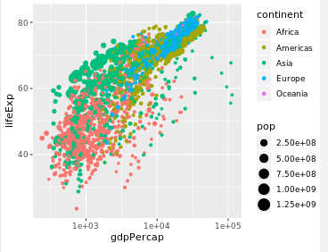
3.4 Faceting
Faceting is a powerful way to understand subsets of your data separately
可以按照条件分类显示数据
facet_wrap(~condi):按照condi来显示数据分类
and size representing population, faceted by year
> ggplot(gapminder,aes(x=gdpPercap,y=lifeExp,colour=continent,size=pop))+
  geom_point()+
  scale_x_log10()
> facet_wrap(~year)
<ggproto object: Class FacetWrap, Facet, gg>
    compute_layout: function
    draw_back: function
    draw_front: function
    draw_labels: function
    draw_panels: function
    finish_data: function
    init_scales: function
    map_data: function
    params: list
    setup_data: function
    setup_params: function
    shrink: TRUE
    train_scales: function
    vars: function
    super:  <ggproto object: Class FacetWrap, Facet, gg>
4.summarize
类似与summary的函数,可以描述性输出。
但是里面的内置函数只有:sum,mean,median,min,max。
 Filter for 1957 then summarize the median life expectancy and the maximum GDP per capita
gapminder%>%filter(year==1957)%>%summarize(
medianLifeExp=median(lifeExp),
maxGdpPercap=max(gdpPercap)
)
5 group_by
分组求解
> # Find median life expectancy and maximum GDP per capita in each continent in 1957
> gapminder%>%filter(year==1957)%>%group_by(continent)%>%summarize(
  medianLifeExp=median(lifeExp),
  maxGdpPercap=max(gdpPercap)
  )
 A tibble: 5 x 3
  continent medianLifeExp maxGdpPercap
  <fct>             <dbl>        <dbl>
1 Africa             40.6        5487.
2 Americas           56.1       14847.
3 Asia               48.3      113523.
4 Europe             67.6       17909.
5 Oceania            70.3       12247.
可以有多个条件进行分组
> # Find median life expectancy and maximum GDP per capita in each continent/year combination
> gapminder%>%group_by(continent,year)%>%summarize(
  medianLifeExp=median(lifeExp),
  maxGdpPercap=max(gdpPercap)
  )
A tibble: 60 x 4
# Groups:   continent [5]
   continent  year medianLifeExp maxGdpPercap
   <fct>     <int>         <dbl>        <dbl>
 1 Africa     1952          38.8        4725.
 2 Africa     1957          40.6        5487.
 3 Africa     1962          42.6        6757.
 4 Africa     1967          44.7       18773.
 5 Africa     1972          47.0       21011.
 6 Africa     1977          49.3       21951.
 7 Africa     1982          50.8       17364.
 8 Africa     1987          51.6       11864.
 9 Africa     1992          52.4       13522.
10 Africa     1997          52.8       14723.
# ... with 50 more rows
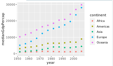
6.expand_limits(y=0)
让y轴从0开始
ibrary(gapminder)
library(dplyr)
library(ggplot2)

# Summarize medianGdpPercap within each continent within each year: by_year_continent
by_year_continent<-gapminder%>%group_by(continent,year)%>%summarize(
medianGdpPercap=median(gdpPercap))

# Plot the change in medianGdpPercap in each continent over time
ggplot(by_year_continent,aes(x=year,y=medianGdpPercap,colour=continent))+geom_point()+
expand_limits(y = 0)
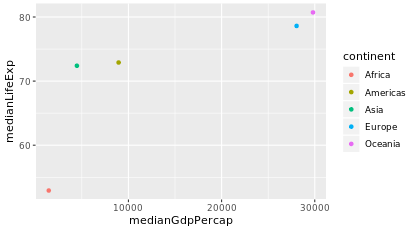
> # Use a scatter plot to compare the median GDP and median life expectancy
> ggplot(by_continent_2007,aes(x=medianLifeExp,y=medianGdpPercap,colour=continent))+geom_point()
> library(gapminder)
> library(dplyr)
> library(ggplot2)
>
> # Summarize the median GDP and median life expectancy per continent in 2007
> by_continent_2007 <- gapminder %>%
    filter(year == 2007) %>%
    group_by(continent) %>%
    summarize(medianGdpPercap = median(gdpPercap),
              medianLifeExp = median(lifeExp))
>
> # Use a scatter plot to compare the median GDP and median life expectancy
> ggplot(by_continent_2007, aes(x = medianGdpPercap, y = medianLifeExp, color = continent)) +
    geom_point()
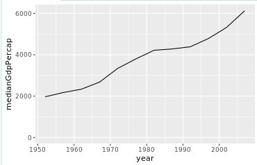
line plot
线图
上面画的都是散点图
library(gapminder)
library(dplyr)
library(ggplot2)

# Summarize the median gdpPercap by year, then save it as by_year
by_year<-gapminder%>%group_by(year)%>%summarize(medianGdpPercap=median(gdpPercap))

# Create a line plot showing the change in medianGdpPercap over time
ggplot(by_year, aes(x = year, y = medianGdpPercap)) +
  geom_line() +
  expand_limits(y = 0)
直线图和散点图的区别就是geom_point()与geom_line()
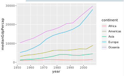
library(ggplot2)
>
> # Summarize the median gdpPercap by year & continent, save as by_year_continent
> by_year_continent<-gapminder%>%group_by(year,continent)%>%summarize(
  medianGdpPercap=median(gdpPercap)
  )
>
> # Create a line plot showing the change in medianGdpPercap by continent over time
> ggplot(by_year_continent,aes(x = year, y = medianGdpPercap,color=continent))+
  geom_line()+
  expand_limits(y = 0)
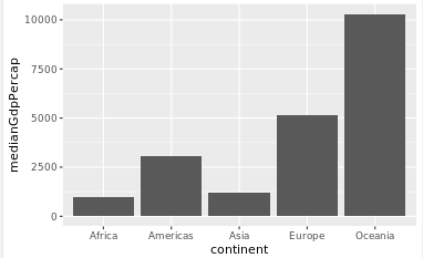
bar plot
 library(gapminder)
> library(dplyr)
> library(ggplot2)
>
> # Summarize the median gdpPercap by year and continent in 1952
> by_continent<-gapminder%>%filter(year==1952)%>%group_by(continent)%>%summarize(
  medianGdpPercap=median(gdpPercap))
>
> # Create a bar plot showing medianGdp by continent
> ggplot(by_continent,aes(x=continent,y=medianGdpPercap))+geom_col()
library(ggplot2)
gapminder_1952 <- gapminder %>%
  filter(year == 1952) %>%
  mutate(pop_by_mil = pop / 1000000)

# Create a histogram of population (pop_by_mil)
ggplot(gapminder_1952,aes(x=pop_by_mil))+
geom_histogram(bins=50)

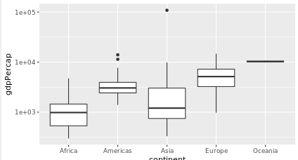
boxplot
# Create a boxplot comparing gdpPercap among continents
> ggplot(gapminder_1952,aes(x=continent,y=gdpPercap))+
  geom_boxplot()+
  scale_y_log10()
> ggplot(gapminder_1952,aes(x=continent,y=gdpPercap))+
  geom_boxplot()+
  scale_y_log10()
ggtitle
如果给表加上标题就用ggtitle("标题名")
gapminder_1952 <- gapminder %>%
    filter(year == 1952)
>
> # Add a title to this graph: "Comparing GDP per capita across continents"
> ggplot(gapminder_1952, aes(x = continent, y = gdpPercap)) +
    geom_boxplot() +
    scale_y_log10()+
    ggtitle("Comparing GDP per capita across continents")