Exercise:Sparse Autoencoder
习题的链接:Exercise:Sparse Autoencoder
注意点:
1、训练样本像素值需要归一化。
因为输出层的激活函数是logistic函数,值域(0,1),
如果训练样本每个像素点没有进行归一化,那将无法进行自编码。
2、训练阶段,向量化实现比for循环实现快十倍。
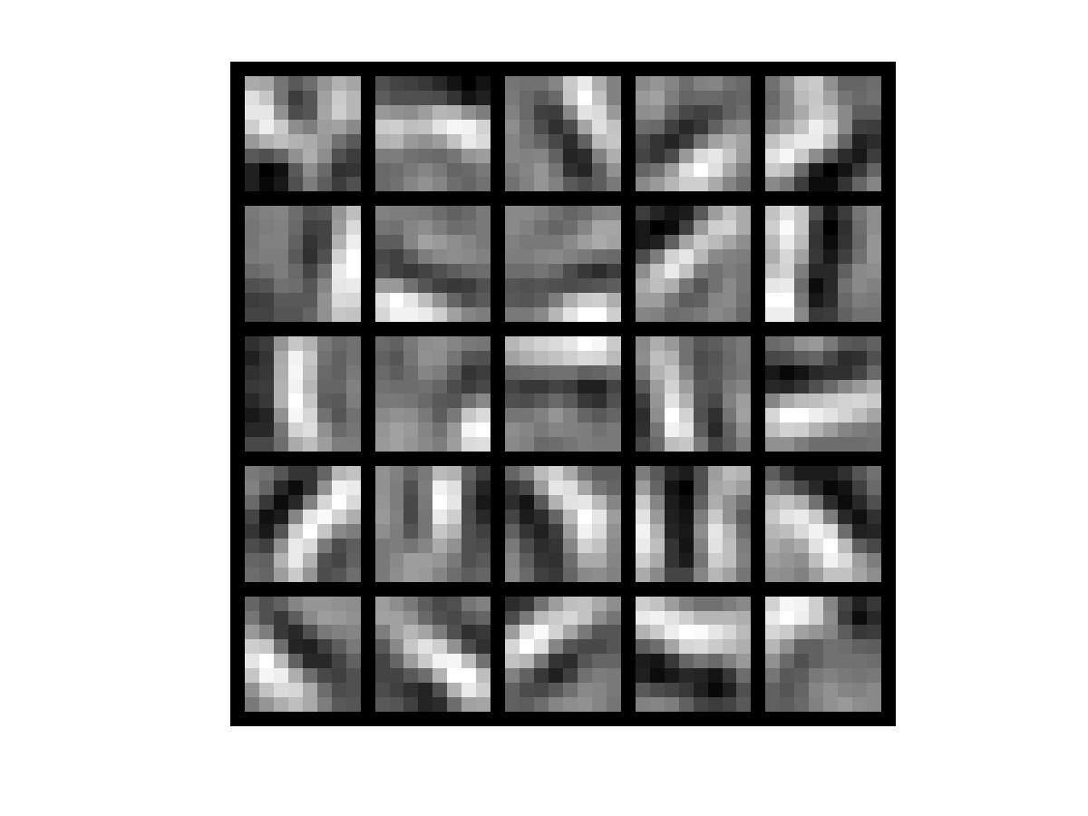
3、最后产生的图片阵列是将W1权值矩阵的转置,每一列作为一张图片。
第i列其实就是最大可能激活第i个隐藏节点的图片xi,再乘以常数因子C(其中C就是W1第i行元素的平方和)。
证明可见:Visualizing a Trained Autoencoder
我的实现:
sampleIMAGES.m
function patches = sampleIMAGES()
% sampleIMAGES
% Returns 10000 patches for training

load IMAGES;    % load images from disk

patchsize = 8;  % we'll use 8x8 patches
numpatches = 10000;

% Initialize patches with zeros.  Your code will fill in this matrix--one
% column per patch, 10000 columns.
patches = zeros(patchsize*patchsize, numpatches);

%% ---------- YOUR CODE HERE --------------------------------------
%  Instructions: Fill in the variable called "patches" using data
%  from IMAGES.
%
%  IMAGES is a 3D array containing 10 images
%  For instance, IMAGES(:,:,6) is a 512x512 array containing the 6th image,
%  and you can type "imagesc(IMAGES(:,:,6)), colormap gray;" to visualize
%  it. (The contrast on these images look a bit off because they have
%  been preprocessed using using "whitening."  See the lecture notes for
%  more details.) As a second example, IMAGES(21:30,21:30,1) is an image
%  patch corresponding to the pixels in the block (21,21) to (30,30) of
%  Image 1

for i=1:numpatches
% generate random row&col number [1, 512-patchsize+1=505]
% generate random IMAGES id [1, 10]
    row = round(1 + rand(1,1)*504);
    col = round(1 + rand(1,1)*504);
    pid = round(1 + rand(1,1)*9);
    patches(:, i) = reshape(IMAGES(row:row+7, col:col+7, pid), patchsize*patchsize, 1);
end

%% ---------------------------------------------------------------
% For the autoencoder to work well we need to normalize the data
% Specifically, since the output of the network is bounded between [0,1]
% (due to the sigmoid activation function), we have to make sure
% the range of pixel values is also bounded between [0,1]
patches = normalizeData(patches);

end


%% ---------------------------------------------------------------
function patches = normalizeData(patches)

% Squash data to [0.1, 0.9] since we use sigmoid as the activation
% function in the output layer

% Remove DC (mean of images).
patches = bsxfun(@minus, patches, mean(patches));

% Truncate to +/-3 standard deviations and scale to -1 to 1
pstd = 3 * std(patches(:));
patches = max(min(patches, pstd), -pstd) / pstd;

% Rescale from [-1,1] to [0.1,0.9]
patches = (patches + 1) * 0.4 + 0.1;

end
computeNumericalGradient.m
function numgrad = computeNumericalGradient(J, theta)
% numgrad = computeNumericalGradient(J, theta)
% theta: a vector of parameters (column vector)
% J: a function that outputs a real-number. Calling y = J(theta) will return the
% function value at theta.

% Initialize numgrad with zeros
numgrad = zeros(size(theta));

%% ---------- YOUR CODE HERE --------------------------------------
% Instructions:
% Implement numerical gradient checking, and return the result in numgrad.
% (See Section 2.3 of the lecture notes.)
% You should write code so that numgrad(i) is (the numerical approximation to) the
% partial derivative of J with respect to the i-th input argument, evaluated at theta.
% I.e., numgrad(i) should be the (approximately) the partial derivative of J with
% respect to theta(i).
%
% Hint: You will probably want to compute the elements of numgrad one at a time.

N = size(theta, 1);
EPSILON = 1e-4;
Identity = eye(N);

for i = 1:N
    numgrad(i,:) = (J(theta + EPSILON * Identity(:, i)) - J(theta - EPSILON * Identity(:, i))) / (2 * EPSILON);
end

%% ---------------------------------------------------------------
end
sparseAutoencoderCost.m
function [cost,grad] = sparseAutoencoderCost(theta, visibleSize, hiddenSize, ...
                                             lambda, sparsityParam, beta, data)

% visibleSize: the number of input units (probably 64)
% hiddenSize: the number of hidden units (probably 25)
% lambda: weight decay parameter
% sparsityParam: The desired average activation for the hidden units (denoted in the lecture
%                           notes by the greek alphabet rho, which looks like a lower-case "p").
% beta: weight of sparsity penalty term
% data: Our 64x10000 matrix containing the training data.  So, data(:,i) is the i-th training example.

% The input theta is a vector (because minFunc expects the parameters to be a vector).
% We first convert theta to the (W1, W2, b1, b2) matrix/vector format, so that this
% follows the notation convention of the lecture notes.

% W1 is a hiddenSize * visibleSize matrix
W1 = reshape(theta(1:hiddenSize*visibleSize), hiddenSize, visibleSize);
% W2 is a visibleSize * hiddenSize matrix
W2 = reshape(theta(hiddenSize*visibleSize+1:2*hiddenSize*visibleSize), visibleSize, hiddenSize);
% b1 is a hiddenSize * 1 vector
b1 = theta(2*hiddenSize*visibleSize+1:2*hiddenSize*visibleSize+hiddenSize);
% b2 is a visible * 1 vector
b2 = theta(2*hiddenSize*visibleSize+hiddenSize+1:end);

% Cost and gradient variables (your code needs to compute these values).
% Here, we initialize them to zeros.
cost = 0;
W1grad = zeros(size(W1));
W2grad = zeros(size(W2));
b1grad = zeros(size(b1));
b2grad = zeros(size(b2));

%% ---------- YOUR CODE HERE --------------------------------------
%  Instructions: Compute the cost/optimization objective J_sparse(W,b) for the Sparse Autoencoder,
%                and the corresponding gradients W1grad, W2grad, b1grad, b2grad.
%
% W1grad, W2grad, b1grad and b2grad should be computed using backpropagation.
% Note that W1grad has the same dimensions as W1, b1grad has the same dimensions
% as b1, etc.  Your code should set W1grad to be the partial derivative of J_sparse(W,b) with
% respect to W1.  I.e., W1grad(i,j) should be the partial derivative of J_sparse(W,b)
% with respect to the input parameter W1(i,j).  Thus, W1grad should be equal to the term
% [(1/m) Delta W^{(1)} + lambda W^{(1)}] in the last block of pseudo-code in Section 2.2
% of the lecture notes (and similarly for W2grad, b1grad, b2grad).
%
% Stated differently, if we were using batch gradient descent to optimize the parameters,
% the gradient descent update to W1 would be W1 := W1 - alpha * W1grad, and similarly for W2, b1, b2.
%

numCases = size(data, 2);

% forward propagation
z2 = W1 * data + repmat(b1, 1, numCases);
a2 = sigmoid(z2);
z3 = W2 * a2 + repmat(b2, 1, numCases);
a3 = sigmoid(z3);

% error
sqrerror = (data - a3) .* (data - a3);
error = sum(sum(sqrerror)) / (2 * numCases);
% weight decay
wtdecay = (sum(sum(W1 .* W1)) + sum(sum(W2 .* W2))) / 2;
% sparsity
rho = sum(a2, 2) ./ numCases;
divergence = sparsityParam .* log(sparsityParam ./ rho) + (1 - sparsityParam) .* log((1 - sparsityParam) ./ (1 - rho));
sparsity = sum(divergence);

cost = error + lambda * wtdecay + beta * sparsity;

% delta3 is a visibleSize * numCases matrix
delta3 = -(data - a3) .* sigmoiddiff(z3);
% delta2 is a hiddenSize * numCases matrix
sparsityterm = beta * (-sparsityParam ./ rho + (1-sparsityParam) ./ (1-rho));
delta2 = (W2' * delta3 + repmat(sparsityterm, 1, numCases)) .* sigmoiddiff(z2);

W1grad = delta2 * data' ./ numCases + lambda * W1;
b1grad = sum(delta2, 2) ./ numCases;

W2grad = delta3 * a2' ./ numCases + lambda * W2;
b2grad = sum(delta3, 2) ./ numCases;

%-------------------------------------------------------------------
% After computing the cost and gradient, we will convert the gradients back
% to a vector format (suitable for minFunc).  Specifically, we will unroll
% your gradient matrices into a vector.

grad = [W1grad(:) ; W2grad(:) ; b1grad(:) ; b2grad(:)];

end

%-------------------------------------------------------------------
% Here's an implementation of the sigmoid function, which you may find useful
% in your computation of the costs and the gradients.  This inputs a (row or
% column) vector (say (z1, z2, z3)) and returns (f(z1), f(z2), f(z3)).

function sigm = sigmoid(x)

    sigm = 1 ./ (1 + exp(-x));
end

function sigmdiff = sigmoiddiff(x)

    sigmdiff = sigmoid(x) .* (1 - sigmoid(x));
end
最终训练结果: