数字图像处理之频域图像增强
by方阳
版权声明:本文为博主原创文章,转载请指明转载地址
http://www.cnblogs.com/fydeblog/p/7069942.html
1. 前言
这篇博客主要讲解频域滤波增强的各类滤波器的实现,并分析不同的滤波器截止频率对频域滤波增强效果的影响。理论的知识还请看书和百度,这里不再复述!
2. 原理说明
(1) 图像的增强可以通过频域滤波来实现,频域低通滤波器滤除高频噪声,频域高通滤波器滤除低频噪声。
(2) 相同类型的滤波器的截止频率不同,对图像的滤除效果也会不同。
3. 实现内容
(1) 选择任意一副图像,对其进行傅里叶变换,在频率域中实现二阶butterworth低通滤波器的平滑作用,截止频率任意设定。显示原始图像和滤波图像。
(2) 选择任意一副图像,对其进行傅里叶变换,在频率域中实现两种不同半径(截止频率)的高斯高通滤波的锐化效果,显示原始图像和滤波图像,及与原图像叠加的高频增强图像。
4. 程序实现及实验结果
(1)butterworth滤波器
参考代码:
I=imread('fig620.jpg');
f=D3_To_D2(I);
PQ=paddedsize(size(f));
[U,V]=dftuv(PQ(1),PQ(2));
D0=0.05*PQ(2);
F=fft2(f,PQ(1),PQ(2));
H=1./(1+((U.^2+V.^2)/(D0^2)).^2);
g=dftfilt(f,H);
figure;
subplot(1,3,1);
imshow(f);
title('原图');
subplot(1,3,2);
imshow(fftshift(H),[]);
title('滤波器频谱');
subplot(1,3,3);
imshow(g,[]);
title('滤波后的图像');
D3_To_D2函数参考代码:
function image_out=D3_To_D2(image_in)
[m,n]=size(image_in);
 n=n/3;%由于我的灰度图像是185x194x3的,所以除了3,你们如果是PxQ的,就不要加了
 A=zeros(m,n);%构造矩阵
 for i=1:m
     for j=1:n
        A(i,j)= image_in(i,j);%填充图像到A
     end
 end
image_out=uint8(A);
paddedsize函数参考代码:
function PQ = paddedsize(AB,CD,~ )
%PADDEDSIZE Computes padded sizes useful for FFT-based filtering.
%   Detailed explanation goes here
if nargin == 1
    PQ = 2*AB;
elseif nargin ==2 && ~ischar(CD)
    PQ = QB +CD -1;
    PQ = 2*ceil(PQ/2);
elseif nargin == 2
    m = max(AB);%maximum dimension

    %Find power-of-2 at least twice m.
    P = 2^nextpow(2*m);
    PQ = [P,P];
elseif nargin == 3
    m = max([AB CD]);%maximum dimension
    P = 2^nextpow(2*m);
    PQ = [P,P];
else
    error('Wrong number of inputs');

end
dftuv函数参考代码:
function [ U,V ] = dftuv( M, N )
%DFTUV 实现频域滤波器的网格函数
%   Detailed explanation goes here
u = 0:(M - 1);
v = 0:(N - 1);
idx = find(u > M/2); %找大于M/2的数据
u(idx) = u(idx) - M; %将大于M/2的数据减去M
idy = find(v > N/2);
v(idy) = v(idy) - N;
[V, U] = meshgrid(v, u);

end
运行结果

(2)高通滤波器
参考代码:
I1=imread('lena.bmp');
f1=D3_To_D2(I1);
PQ1=paddedsize(size(f1));
D0_1=0.05*PQ(1);
D0_2=0.1*PQ(1);
H1=hpfilter('gaussian',PQ1(1),PQ1(2),D0_1);
H2=hpfilter('gaussian',PQ1(1),PQ1(2),D0_2);
g1=dftfilt(f1,H1);
g2=dftfilt(f1,H2);
H1=0.5+2*H1;
H2=0.5+2*H2;
g3=dftfilt(f1,H1);
g4=dftfilt(f1,H2);
g3=histeq(gscale(g3),256);
g4=histeq(gscale(g4),256);
figure;
subplot(2,3,1);
imshow(f1);
title('原图');
subplot(2,3,2);
imshow(g1,[]);
title('滤波后的图像-系数0.05');
subplot(2,3,3);
imshow(g2,[]);
title('滤波后的图像-系数0.1');
subplot(2,3,4);
imshow(g3,[]);
title('增强后的图像-系数0.05');
subplot(2,3,5);
imshow(g4,[]);
title('增强后的图像-系数0.1');
hpfilter函数参考代码:
function H = hpfilter(type, M, N, D0, n)
if nargin == 4
    n = 1;
end
hlp = lpfilter(type, M, N, D0, n);
H = 1 - hlp;
hpfilter中的lpfilter参考代码:
function [ H, D ] = lpfilter( type,M,N,D0,n )
%LPFILTER creates the transfer function of a lowpass filter.
%   Detailed explanation goes here

%use function dftuv to set up the meshgrid arrays needed for computing
%the required distances.
[U, V] = dftuv(M,N);

%compute the distances D(U,V)
D = sqrt(U.^2 + V.^2);

%begin filter computations
switch type
    case 'ideal'
        H = double(D <= D0);
    case 'btw'
        if nargin == 4
            n = 1;
        end
        H = 1./(1+(D./D0).^(2*n));
    case 'gaussian'
        H = exp(-(D.^2)./(2*(D0^2)));
    otherwise
        error('Unkown filter type');

end
gscale函数参考代码:
function g = gscale(f, varargin)
%GSCALE Scales the intensity of the input image.
%   G = GSCALE(F, 'full8') scales the intensities of F to the full
%   8-bit intensity range [0, 255].  This is the default if there is
%   only one input argument.
%
%   G = GSCALE(F, 'full16') scales the intensities of F to the full
%   16-bit intensity range [0, 65535].
%
%   G = GSCALE(F, 'minmax', LOW, HIGH) scales the intensities of F to
%   the range [LOW, HIGH]. These values must be provided, and they
%   must be in the range [0, 1], independently of the class of the
%   input. GSCALE performs any necessary scaling. If the input is of
%   class double, and its values are not in the range [0, 1], then
%   GSCALE scales it to this range before processing.
%
%   The class of the output is the same as the class of the input.

%   Copyright 2002-2004 R. C. Gonzalez, R. E. Woods, & S. L. Eddins
%   Digital Image Processing Using MATLAB, Prentice-Hall, 2004
%   $Revision: 1.5 $  $Date: 2003/11/21 14:36:09 $

if length(varargin) == 0 % If only one argument it must be f.
   method = 'full8';
else
   method = varargin{1};
end

if strcmp(class(f), 'double') & (max(f(:)) > 1 | min(f(:)) < 0)
   f = mat2gray(f);
end

% Perform the specified scaling.
switch method
case 'full8'
   g = im2uint8(mat2gray(double(f)));
case 'full16'
   g = im2uint16(mat2gray(double(f)));
case 'minmax'
   low = varargin{2}; high = varargin{3};
   if low > 1 | low < 0 | high > 1 | high < 0
      error('Parameters low and high must be in the range [0, 1].')
   end
   if strcmp(class(f), 'double')
      low_in = min(f(:));
      high_in = max(f(:));
   elseif strcmp(class(f), 'uint8')
      low_in = double(min(f(:)))./255;
      high_in = double(max(f(:)))./255;
   elseif strcmp(class(f), 'uint16')
      low_in = double(min(f(:)))./65535;
      high_in = double(max(f(:)))./65535;
   end
   % imadjust automatically matches the class of the input.
   g = imadjust(f, [low_in high_in], [low high]);
otherwise
   error('Unknown method.')
end
运行结果:
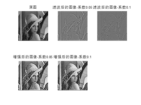
五.结果分析
(1)由第一个图可以看出,图像经过低通滤波器,图像的高频分量滤掉了,图像变得平滑。
(2)由第二个图可以看出,图像不同的截止频率,出来的图像也不同,系数小的效果强。