入口,sql
  /**
   * Executes a SQL query using Spark, returning the result as a `DataFrame`.
   * This API eagerly runs DDL/DML commands, but not for SELECT queries.
   *
   * @since 2.0.0
   */
  def sql(sqlText: String): DataFrame = withActive {
    val tracker = new QueryPlanningTracker // 记录执行过程
    val plan = tracker.measurePhase(QueryPlanningTracker.PARSING) { // parse,返回LogicalPlan
      sessionState.sqlParser.parsePlan(sqlText)
    }
    Dataset.ofRows(self, plan, tracker)
  }
ofRows
  /** A variant of ofRows that allows passing in a tracker so we can track query parsing time. */
  def ofRows(sparkSession: SparkSession, logicalPlan: LogicalPlan, tracker: QueryPlanningTracker)
    : DataFrame = sparkSession.withActive { //把当前session设置成active
    val qe = new QueryExecution(sparkSession, logicalPlan, tracker) //生成QueryExecution对象
    qe.assertAnalyzed()  //Analyzed,做AST的resolve
    new Dataset[Row](qe, RowEncoder(qe.analyzed.schema)) //最终生成Dataset
  }
}
Analyze
  lazy val analyzed: LogicalPlan = executePhase(QueryPlanningTracker.ANALYSIS) {
    // We can't clone `logical` here, which will reset the `_analyzed` flag.
    sparkSession.sessionState.analyzer.executeAndCheck(logical, tracker)
  }
Analyse主要做的是resolve,AST到logical plan
这里和后面的optimization一样,也是基于一套Rule系统,所以Analyzer继承于RuleExecutor
最终调用到RuleExecutor的execute,
  /**
   * Executes the batches of rules defined by the subclass. The batches are executed serially
   * using the defined execution strategy. Within each batch, rules are also executed serially.
   */
  def execute(plan: TreeType): TreeType = {
    var curPlan = plan

    batches.foreach { batch =>   //对于每个batch
      val batchStartPlan = curPlan
      var iteration = 1
      var lastPlan = curPlan
      var continue = true    //默认true

      // Run until fix point (or the max number of iterations as specified in the strategy.
      while (continue) {
        curPlan = batch.rules.foldLeft(curPlan) {
          case (plan, rule) =>
            val startTime = System.nanoTime()
            val result = rule(plan)
            val runTime = System.nanoTime() - startTime
            val effective = !result.fastEquals(plan)
            //......
            result
        }
        iteration += 1
        if (iteration > batch.strategy.maxIterations) { //对于batch的maxIterations如果达到,跳出batch
          // ......
          continue = false
        }

        if (curPlan.fastEquals(lastPlan)) {
          logTrace(
            s"Fixed point reached for batch ${batch.name} after ${iteration - 1} iterations.")
          continue = false
        }
        lastPlan = curPlan
      }

      planChangeLogger.logBatch(batch.name, batchStartPlan, curPlan)
    }
    planChangeLogger.logMetrics(RuleExecutor.getCurrentMetrics() - beforeMetrics)

    curPlan
  }
整体的逻辑比较简单,就是依次执行每个batch中的每个rule,每个batch本身有个maxIterations,规定这个batch可以被迭代的最大次数
看下,analyzer中定义的rules,
其中,once就是执行一次,fixedPoint就是执行多次到maxIterations,大部分都是resolution
  override def batches: Seq[Batch] = Seq(
    Batch("Substitution", fixedPoint,
      OptimizeUpdateFields,
      CTESubstitution,
      WindowsSubstitution,
      EliminateUnions,
      SubstituteUnresolvedOrdinals),
    Batch("Disable Hints", Once,
      new ResolveHints.DisableHints),
    Batch("Hints", fixedPoint,
      ResolveHints.ResolveJoinStrategyHints,
      ResolveHints.ResolveCoalesceHints),
    Batch("Simple Sanity Check", Once,
      LookupFunctions),
    Batch("Resolution", fixedPoint,
      ResolveTableValuedFunctions ::
      ResolveNamespace(catalogManager) ::
      new ResolveCatalogs(catalogManager) ::
      ResolveUserSpecifiedColumns ::
      ResolveInsertInto ::
      ResolveRelations ::
      ResolveTables ::
      ......
      TypeCoercion.typeCoercionRules ++
      extendedResolutionRules : _*),
    Batch("Apply Char Padding", Once,
      ApplyCharTypePadding),
    Batch("Post-Hoc Resolution", Once,
      Seq(ResolveNoopDropTable) ++
      postHocResolutionRules: _*),
    Batch("Normalize Alter Table", Once, ResolveAlterTableChanges),
    Batch("Remove Unresolved Hints", Once,
      new ResolveHints.RemoveAllHints),
    Batch("Nondeterministic", Once,
      PullOutNondeterministic),
    Batch("UDF", Once,
      HandleNullInputsForUDF,
      ResolveEncodersInUDF),
    Batch("UpdateNullability", Once,
      UpdateAttributeNullability),
    Batch("Subquery", Once,
      UpdateOuterReferences),
    Batch("Cleanup", fixedPoint,
      CleanupAliases)
  )
简单的看下,其中的一个rule,
主要就是利用Scala的Pattern matching特性进行匹配和逻辑处理
  /**
   * Resolve table relations with concrete relations from v2 catalog.
   *
   * [[ResolveRelations]] still resolves v1 tables.
   */
  object ResolveTables extends Rule[LogicalPlan] {
    def apply(plan: LogicalPlan): LogicalPlan = ResolveTempViews(plan).resolveOperatorsUp {
      case u: UnresolvedRelation =>
        lookupV2Relation(u.multipartIdentifier, u.options, u.isStreaming) //如果UnresolvedRelation, 需要lookup
          .map { relation =>
            val (catalog, ident) = relation match {
              case ds: DataSourceV2Relation => (ds.catalog, ds.identifier.get)
              case s: StreamingRelationV2 => (s.catalog, s.identifier.get)
            }
            SubqueryAlias(catalog.get.name +: ident.namespace :+ ident.name, relation)
          }.getOrElse(u)

      case u @ UnresolvedTable(NonSessionCatalogAndIdentifier(catalog, ident), _) =>  //@表示变量binding
        CatalogV2Util.loadTable(catalog, ident)
          .map(ResolvedTable(catalog.asTableCatalog, ident, _))
          .getOrElse(u)
在Analyze完成后,将Query Execution封装在Dateset中,
什么是Dataset?
/**
 * A Dataset is a strongly typed collection of domain-specific objects that can be transformed
 * in parallel using functional or relational operations. Each Dataset also has an untyped view
 * called a `DataFrame`, which is a Dataset of [[Row]].
Dataset[T],一个泛型的抽象
Dataset[Row],叫做DataFrame,也就是一种确定类型的Dataset,数据表的抽象。
 * Operations available on Datasets are divided into transformations and actions. Transformations
 * are the ones that produce new Datasets, and actions are the ones that trigger computation and
 * return results. Example transformations include map, filter, select, and aggregate (`groupBy`).
 * Example actions count, show, or writing data out to file systems.
 *
 * Datasets are "lazy", i.e. computations are only triggered when an action is invoked. Internally,
 * a Dataset represents a logical plan that describes the computation required to produce the data.
 * When an action is invoked, Spark's query optimizer optimizes the logical plan and generates a
 * physical plan for efficient execution in a parallel and distributed manner. To explore the
 * logical plan as well as optimized physical plan, use the `explain` function.
Operations分为transformations and actions
Transformation得到的仍然是Dataset,Action是从Dataset中取出最终结果
所以Trans是Lazy的,Action才会触发真正的执行,这个是Spark的基本特点,以前RDD也是这样
 * To efficiently support domain-specific objects, an [[Encoder]] is required. The encoder maps
 * the domain specific type `T` to Spark's internal type system. For example, given a class `Person`
 * with two fields, `name` (string) and `age` (int), an encoder is used to tell Spark to generate
 * code at runtime to serialize the `Person` object into a binary structure. This binary structure
 * often has much lower memory footprint as well as are optimized for efficiency in data processing
 * (e.g. in a columnar format). To understand the internal binary representation for data, use the
 * `schema` function.
domain-specific,就是UDT,用户定义类型
所以要提供Encoder,用于用户类型到Spark类型structure的转换
在具有DataSet后,调用actions,让他真正执行,比如collect,count
会调用withAction
withAction
  /**
   * Wrap a Dataset action to track the QueryExecution and time cost, then report to the
   * user-registered callback functions.
   */
  private def withAction[U](name: String, qe: QueryExecution)(action: SparkPlan => U) = {
    SQLExecution.withNewExecutionId(qe, Some(name)) {
      qe.executedPlan.resetMetrics()
      action(qe.executedPlan) //调用executedPlan
    }
  }
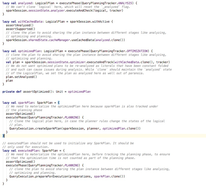
在QueryExecution中,会依次从,
executedPlan,sparkPlan,optimizedPlan,withCachedData
withCacheData是避免重复优化,所以主要是3步,
Optimizer
机制和Analyzer是一样的,RBO
就不列出具体的rules,看其中的一个ruleBatch
Batch("Join Reorder", FixedPoint(1),
      CostBasedJoinReorder)
CostBasedJoinReorder
不同于cascade模型,对于join的交换和结合律都是一个rule
这里是用一个rule,完成整个joinorder的选择,所以逻辑都封装在这个rule中
object CostBasedJoinReorder extends Rule[LogicalPlan] with PredicateHelper {

  def apply(plan: LogicalPlan): LogicalPlan = {
    if (!conf.cboEnabled || !conf.joinReorderEnabled) {
      plan
    } else {
      val result = plan transformDown {
        // Start reordering with a joinable item, which is an InnerLike join with conditions.
        // Avoid reordering if a join hint is present.
        case j @ Join(_, _, _: InnerLike, Some(cond), JoinHint.NONE) =>  //Pattern Matching
          reorder(j, j.output)
        case p @ Project(projectList, Join(_, _, _: InnerLike, Some(cond), JoinHint.NONE))
          if projectList.forall(_.isInstanceOf[Attribute]) =>
          reorder(p, p.output)
      }
      // After reordering is finished, convert OrderedJoin back to Join.
      result transform {
        case OrderedJoin(left, right, jt, cond) => Join(left, right, jt, cond, JoinHint.NONE)
      }
    }
  }

  private def reorder(plan: LogicalPlan, output: Seq[Attribute]): LogicalPlan = {
    val (items, conditions) = extractInnerJoins(plan)
    val result =
      // Do reordering if the number of items is appropriate and join conditions exist.
      // We also need to check if costs of all items can be evaluated.
      if (items.size > 2 && items.size <= conf.joinReorderDPThreshold && conditions.nonEmpty &&
          items.forall(_.stats.rowCount.isDefined)) {
        JoinReorderDP.search(conf, items, conditions, output) //DP动态规划,找到最优的Join order
      } else {
        plan
      }
    // Set consecutive join nodes ordered.
    replaceWithOrderedJoin(result)
  }
JoinReorderDP
- bottomup,自底向上逐级
- 对于每个子集仅仅保留bestplan,非完全的DP
E.g., for 3-way joins, we keep only the best plan for items {A, B, C} among plans (A J B) J C, (A J C) J B and (B J C) J A.
- 只考虑有join condition的,prune cartesian product candidates,参考下面的例子
/**
 * Reorder the joins using a dynamic programming algorithm. This implementation is based on the
 * paper: Access Path Selection in a Relational Database Management System.
 * https://dl.acm.org/doi/10.1145/582095.582099
 *
 * First we put all items (basic joined nodes) into level 0, then we build all two-way joins
 * at level 1 from plans at level 0 (single items), then build all 3-way joins from plans
 * at previous levels (two-way joins and single items), then 4-way joins ... etc, until we
 * build all n-way joins and pick the best plan among them.
 *
 * When building m-way joins, we only keep the best plan (with the lowest cost) for the same set
 * of m items. E.g., for 3-way joins, we keep only the best plan for items {A, B, C} among
 * plans (A J B) J C, (A J C) J B and (B J C) J A.
 * We also prune cartesian product candidates when building a new plan if there exists no join
 * condition involving references from both left and right. This pruning strategy significantly
 * reduces the search space.
 * E.g., given A J B J C J D with join conditions A.k1 = B.k1 and B.k2 = C.k2 and C.k3 = D.k3,
 * plans maintained for each level are as follows:
 * level 0: p({A}), p({B}), p({C}), p({D})
 * level 1: p({A, B}), p({B, C}), p({C, D})
 * level 2: p({A, B, C}), p({B, C, D})
 * level 3: p({A, B, C, D})
 * where p({A, B, C, D}) is the final output plan.
 *
 * For cost evaluation, since physical costs for operators are not available currently, we use
 * cardinalities and sizes to compute costs.
 */
object JoinReorderDP extends PredicateHelper with Logging {
SparkPlan
逻辑plan转化成物理plan
QueryExecution.createSparkPlan(sparkSession, planner, optimizedPlan.clone())
调用planner.plan
  /**
   * Transform a [[LogicalPlan]] into a [[SparkPlan]].
   *
   * Note that the returned physical plan still needs to be prepared for execution.
   */
  def createSparkPlan(
      sparkSession: SparkSession,
      planner: SparkPlanner,
      plan: LogicalPlan): SparkPlan = {
    // TODO: We use next(), i.e. take the first plan returned by the planner, here for now,
    //       but we will implement to choose the best plan.
    planner.plan(ReturnAnswer(plan)).next()
  }
QueryPlanner
遍历Strategies里面的每个strategy,应用到逻辑plan上
abstract class QueryPlanner[PhysicalPlan <: TreeNode[PhysicalPlan]] {
  /** A list of execution strategies that can be used by the planner */
  def strategies: Seq[GenericStrategy[PhysicalPlan]]

  def plan(plan: LogicalPlan): Iterator[PhysicalPlan] = {
    // Obviously a lot to do here still...

    // Collect physical plan candidates.
    val candidates = strategies.iterator.flatMap(_(plan))
strategies,可以参考在SparkPlanner上给出的一个例子,当然你可以给出任意的strategy的组合
  override def strategies: Seq[Strategy] =
    experimentalMethods.extraStrategies ++
      extraPlanningStrategies ++ (
      LogicalQueryStageStrategy ::
      PythonEvals ::
      new DataSourceV2Strategy(session) ::
      FileSourceStrategy ::
      DataSourceStrategy ::
      SpecialLimits ::
      Aggregation ::
      Window ::
      JoinSelection ::
      InMemoryScans ::
      BasicOperators :: Nil)
看下其中的JoinSelection
选择join的实现,这里支持若干种的join的实现,
  /**
   * Select the proper physical plan for join based on join strategy hints, the availability of
   * equi-join keys and the sizes of joining relations. Below are the existing join strategies,
   * their characteristics and their limitations.
   *
   * - Broadcast hash join (BHJ):
   *     Only supported for equi-joins, while the join keys do not need to be sortable.
   *     Supported for all join types except full outer joins.
   *     BHJ usually performs faster than the other join algorithms when the broadcast side is
   *     small. However, broadcasting tables is a network-intensive operation and it could cause
   *     OOM or perform badly in some cases, especially when the build/broadcast side is big.
   *
   * - Shuffle hash join:
   *     Only supported for equi-joins, while the join keys do not need to be sortable.
   *     Supported for all join types.
   *     Building hash map from table is a memory-intensive operation and it could cause OOM
   *     when the build side is big.
   *
   * - Shuffle sort merge join (SMJ):
   *     Only supported for equi-joins and the join keys have to be sortable.
   *     Supported for all join types.
   *
   * - Broadcast nested loop join (BNLJ):
   *     Supports both equi-joins and non-equi-joins.
   *     Supports all the join types, but the implementation is optimized for:
   *       1) broadcasting the left side in a right outer join;
   *       2) broadcasting the right side in a left outer, left semi, left anti or existence join;
   *       3) broadcasting either side in an inner-like join.
   *     For other cases, we need to scan the data multiple times, which can be rather slow.
   *
   * - Shuffle-and-replicate nested loop join (a.k.a. cartesian product join):
   *     Supports both equi-joins and non-equi-joins.
   *     Supports only inner like joins.
   */
  object JoinSelection extends Strategy
    with PredicateHelper
    with JoinSelectionHelper {
看下核心的实现apply
当匹配到EquiJoin的时候,依次根据hint创建各种join的实现
如果最后发现无hint,调用createJoinWithoutHint
def apply(plan: LogicalPlan): Seq[SparkPlan] = plan match {

      // If it is an equi-join, we first look at the join hints w.r.t. the following order:
      //   1. broadcast hint: pick broadcast hash join if the join type is supported. If both sides
      //      have the broadcast hints, choose the smaller side (based on stats) to broadcast.
      //   2. sort merge hint: pick sort merge join if join keys are sortable.
      //   3. shuffle hash hint: We pick shuffle hash join if the join type is supported. If both
      //      sides have the shuffle hash hints, choose the smaller side (based on stats) as the
      //      build side.
      //   4. shuffle replicate NL hint: pick cartesian product if join type is inner like.
      //
      // If there is no hint or the hints are not applicable, we follow these rules one by one:
      //   1. Pick broadcast hash join if one side is small enough to broadcast, and the join type
      //      is supported. If both sides are small, choose the smaller side (based on stats)
      //      to broadcast.
      //   2. Pick shuffle hash join if one side is small enough to build local hash map, and is
      //      much smaller than the other side, and `spark.sql.join.preferSortMergeJoin` is false.
      //   3. Pick sort merge join if the join keys are sortable.
      //   4. Pick cartesian product if join type is inner like.
      //   5. Pick broadcast nested loop join as the final solution. It may OOM but we don't have
      //      other choice.
      case j @ ExtractEquiJoinKeys(joinType, leftKeys, rightKeys, nonEquiCond, left, right, hint) =>
        createBroadcastHashJoin(true)
          .orElse { if (hintToSortMergeJoin(hint)) createSortMergeJoin() else None }
          .orElse(createShuffleHashJoin(true))
          .orElse { if (hintToShuffleReplicateNL(hint)) createCartesianProduct() else None }
          .getOrElse(createJoinWithoutHint())
具体看下,createBroadcastHashJoin
        def createBroadcastHashJoin(onlyLookingAtHint: Boolean) = {
          getBroadcastBuildSide(left, right, joinType, hint, onlyLookingAtHint, conf).map {
            buildSide =>
              Seq(joins.BroadcastHashJoinExec(
                leftKeys,
                rightKeys,
                joinType,
                buildSide,
                nonEquiCond,
                planLater(left),
                planLater(right)))
          }
        }
getBroadcastBuildSide,决定build哪一边,对left还是right进行broadcast,会根据hint和size进行选择
BroadcastHashJoinExec
/**
 * Performs an inner hash join of two child relations.  When the output RDD of this operator is
 * being constructed, a Spark job is asynchronously started to calculate the values for the
 * broadcast relation.  This data is then placed in a Spark broadcast variable.  The streamed
 * relation is not shuffled.
 */
case class BroadcastHashJoinExec(
    leftKeys: Seq[Expression],
    rightKeys: Seq[Expression],
    joinType: JoinType,
    buildSide: BuildSide,
    condition: Option[Expression],
    left: SparkPlan,
    right: SparkPlan,
    isNullAwareAntiJoin: Boolean = false)
  extends HashJoin with CodegenSupport {
doExecute,执行
join的左右两表,分为buildPlan和streamedPlan
执行完,返回的结果是RDD
  protected override def doExecute(): RDD[InternalRow] = {
    val numOutputRows = longMetric("numOutputRows")

    val broadcastRelation = buildPlan.executeBroadcast[HashedRelation]() //由buildPlan生成Broadcast

    streamedPlan.execute().mapPartitions { streamedIter =>
      val hashed = broadcastRelation.value.asReadOnlyCopy()
      join(streamedIter, hashed, numOutputRows) //join
    }
executedPlan
执行前做一些准备工作
QueryExecution.prepareForExecution(preparations, sparkPlan.clone())
准备工作,包含增加shuffle操作和内部的row格式转换
  /**
   * Prepares a planned [[SparkPlan]] for execution by inserting shuffle operations and internal
   * row format conversions as needed.
   */
  private[execution] def prepareForExecution(
      preparations: Seq[Rule[SparkPlan]],
      plan: SparkPlan): SparkPlan = {
    val planChangeLogger = new PlanChangeLogger[SparkPlan]()
    val preparedPlan = preparations.foldLeft(plan) { case (sp, rule) =>
      val result = rule.apply(sp)
      planChangeLogger.logRule(rule.ruleName, sp, result)
      result
    }
    planChangeLogger.logBatch("Preparations", plan, preparedPlan)
    preparedPlan
  }
对于preparations,调用foldLeft,前一次调用的result作为input
preparations包含,
  /**
   * Construct a sequence of rules that are used to prepare a planned [[SparkPlan]] for execution.
   * These rules will make sure subqueries are planned, make use the data partitioning and ordering
   * are correct, insert whole stage code gen, and try to reduce the work done by reusing exchanges
   * and subqueries.
   */
  private[execution] def preparations(
      sparkSession: SparkSession,
      adaptiveExecutionRule: Option[InsertAdaptiveSparkPlan] = None): Seq[Rule[SparkPlan]] = {
    // `AdaptiveSparkPlanExec` is a leaf node. If inserted, all the following rules will be no-op
    // as the original plan is hidden behind `AdaptiveSparkPlanExec`.
    adaptiveExecutionRule.toSeq ++
    Seq(
      CoalesceBucketsInJoin,
      PlanDynamicPruningFilters(sparkSession),
      PlanSubqueries(sparkSession),
      RemoveRedundantProjects,
      EnsureRequirements,
      // `RemoveRedundantSorts` needs to be added after `EnsureRequirements` to guarantee the same
      // number of partitions when instantiating PartitioningCollection.
      RemoveRedundantSorts,
      DisableUnnecessaryBucketedScan,
      ApplyColumnarRulesAndInsertTransitions(sparkSession.sessionState.columnarRules),
      CollapseCodegenStages(),
      ReuseExchange,
      ReuseSubquery
    )
  }