欠拟合与过拟合(underfiting、overfiting)
欠拟合(举例:7个样本点用1次项假设拟合房屋价格和面积的关系,损失了2次成分)
过拟合(举例:7个样本点用6次项假设拟合房屋价格和面积的关系)
参数学习算法(parametric learning algorithm)
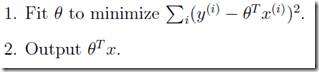
线性回归
非参数学习算法(non-parametric learning algorithm)
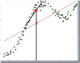
局部加权回归(Locally weighted linear regression、LWR)
由于参数学习算法依赖特征的选择(1次?2次?)
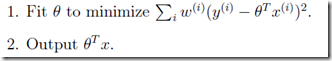
添加了一个wi权重项,值越大,它所对应的对结果的影响越大,反之越小。
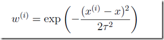
该公式与高斯函数相似,但是没有任何关系,只是这个公式在这里很好用。是波长参数,控制了权值随距离的下降速率(成反比)。
所谓参数学习算法它有固定的明确的参数,参数一旦确定,就不会改变了,我们不需要在保留训练集中的训练样本。
而非参数学习算法,每进行一次预测,就需要重新学习一组,是变化的,所以需要一直保留训练样本。
也就是说,当训练集的容量较大时,非参数学习算法需要占用更多的存储空间,计算速度也较慢。
概率解释
- 为什么使用最小二乘?

假设误差是IID(独立同分布)。

高斯密度函数
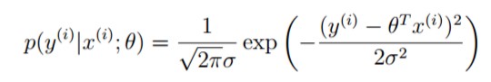
这里使用分号是因为参数theta是一个存在的值,不是随机变量,读作“以theta为参数的概率”。这是采用了频率学派的观点,而非贝叶斯学派。

前者是参数的似然性L(theta),这里看作是theta的概率密度函数;后者是数据的概率,在这里是等价的。

- 补充:极大似然估计(MLE)
1.选择theta是似然性最大化,或者选择参数是数据出现的概率最大化。
2. 取对数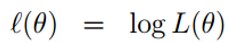
3. 使对数似然最大化
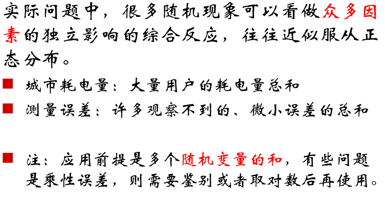
- 补充:中心极限定理
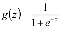
Logistic回归
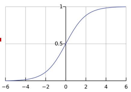


此处可以使用梯度上升算法
θ := θ + α ▼θ l(θ)

Logistic回归参数的学习规则与线性回归有完全相同的形式,前者是梯度上升(基于概率P(y|x;θ)),后者是梯度下降(基于最小二乘)。是完全不同的学习算法。
感知器算法(PLA、Perceptron Learning Algorithm)
感知器算法强迫函数输出为{0,1}的离散值而不是概率。其预测函数为:
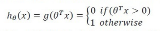
参数θ的更新规则为:
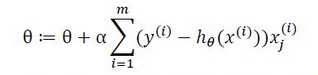
规则看起来与logistic回归相同,其实是完全不同的算法,而且更加简单。
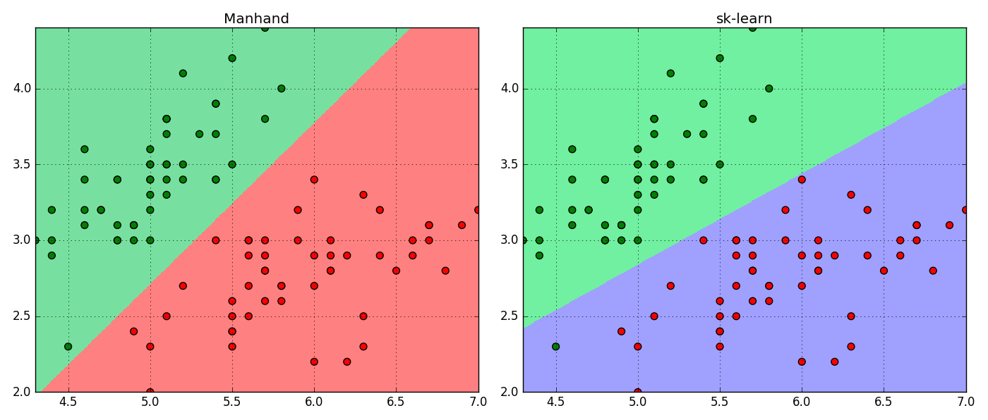
代码实践(Logistic回归)
# -*- coding: utf-8 -*-
import numpy as np
import matplotlib as mpl
import matplotlib.pyplot as plt
from sklearn.linear_model import LogisticRegression
def sigmoid( X , theta ):
    z = np.dot( X , theta.T )
    return 1 / ( 1 + np.exp( -z ) )
def LR( X , y , times=400 , alpha=0.01 ):
    X = np.c_[ (np.ones(len(X)) , X )]
    theta = np.zeros(len(X[0])).T
    for i in range(times):
        h = sigmoid(X , theta)
        theta += alpha * np.dot( ( y - h ).T , X )
    return theta
def Predict( X , theta ):
    X = np.c_[ (np.ones(len(X)) , X )]
    return (sigmoid(X , theta) + 0.5).astype(np.int32)

df = np.loadtxt(r'C:UsersLoveDMRDesktop8.iris.data', delimiter=',' , converters = { 4: lambda t : {'Iris-setosa':0,'Iris-versicolor':1,'Iris-virginica':2}[t] } );
df = df[df[:,4] != 2]
X , y = np.split(df,(4,), axis=1)
X =X[:,:2]
y = y[:,0]
# sklearn
model = LogisticRegression()
model.fit(X,y)
print model.intercept_ , model.coef_
# manhand
theta = LR(X , y , 100000 )
print theta
plt.figure(figsize=(14,6))
plt.subplot(121)
N, M = 500, 500     # 横纵各采样多少个值
x1_min, x1_max = X[:, 0].min(), X[:, 0].max()   # 第0列的范围
x2_min, x2_max = X[:, 1].min(), X[:, 1].max()   # 第1列的范围
t1 = np.linspace(x1_min, x1_max, N)
t2 = np.linspace(x2_min, x2_max, M)
x1, x2 = np.meshgrid(t1, t2)                    # 生成网格采样点
x_test = np.stack((x1.flat, x2.flat), axis=1)   # 测试点
cm_light = mpl.colors.ListedColormap(['#77E0A0', '#FF8080'])
cm_dark = mpl.colors.ListedColormap(['g', 'r'])
y_hat = Predict(x_test,theta)                  # 预测值
y_hat = y_hat.reshape(x1.shape)                 # 使之与输入的形状相同
plt.pcolormesh(x1, x2, y_hat, cmap=cm_light)     # 预测值的显示
plt.scatter(X[:, 0], X[:, 1], c=y, edgecolors='k', s=50, cmap=cm_dark)    # 样本的显示
plt.xlim(x1_min, x1_max)
plt.ylim(x2_min, x2_max)
plt.title('Manhand')
plt.tight_layout()
plt.grid()
plt.subplot(122)
cm_light = mpl.colors.ListedColormap(['#70F0A0', '#A0A0FF'])
cm_dark = mpl.colors.ListedColormap(['g', 'r'])
y_skhat = model.predict(x_test)                  # 预测值
y_skhat = y_skhat.reshape(x1.shape)                 # 使之与输入的形状相同
plt.pcolormesh(x1, x2, y_skhat , cmap=cm_light)     # 预测值的显示
plt.scatter(X[:, 0], X[:, 1], c=y, edgecolors='k', s=50, cmap=cm_dark)    # 样本的显示
plt.xlim(x1_min, x1_max)
plt.ylim(x2_min, x2_max)
plt.title('sk-learn')
plt.tight_layout()
plt.grid()
#plt.savefig('2.png')
plt.show()