% 已知圆心和半径画圆:参考:https://blog.csdn.net/ZLK961543260/article/details/70216089
% 对比三种画圆方法,运算时长对比如下
% viscircle:0.22;比较快
% rectangle:0.21;比较快
% function:0.39:慢

[Type Sheet Format]=xlsfinfo('现状OD数据及其他数据.xls');
OD=xlsread('现状OD数据及其他数据.xls',Sheet{1});
center_area=xlsread('现状OD数据及其他数据.xls',Sheet{2});

x_pos=center_area(:,4);   %数据第四列为x坐标(米)
y_pos=center_area(:,5);   %数据第五列为y坐标(米)
area=center_area(:,3);    %数据第3列为面积(平方米):注意与x,y的坐标对应
r_all=sqrt(area/pi);      %计算节点覆盖半径,为后文画圆做准备
nanbool=isnan(r_all);     %数据1到4行为四个物流园区,通过r为nan,提取出四个物流园区
first_node_num=length(find(nanbool==1)); %统计物流园区个数
r_index=find(nanbool==0,1);              %节点开始的行数index
r=r_all(r_index:end);                    %r存储节点的覆盖半径
jam_coef=center_area(r_index:end,6);     %数据第六列为交通拥堵系数,只有节点才有,具体在散点图中的标注用text实现,
% 具体标注可参考https://zhidao.baidu.com/question/924100748051179779.html
% 散点图颜色可参考:https://zhidao.baidu.com/question/521200141403285445.html?qbl=relate_question_1&word=matlabscatter%B1%EA%D7%A2
% 具体标注和颜色还未完善

% 方法一:viscircle
%用viscircle画节点的覆盖范围,用scatter画物流园区和节点
x_2_pos=x_pos(r_index:end);     %节点x
y_2_pos=y_pos(r_index:end);     %节点y
centers=[x_2_pos,y_2_pos];      %节点圆心位置
tic
fig1=figure
colors = {'b','r','g','y','k'};
%定义colors,后文画图方便,也可以只是掉,直接在后文加入'k','g'等,具体可查询matlab画图颜色标记表示
viscircles(centers,r,'color',colors{1});    %matlab自带函数:已知圆心和半径画圆
hold on
scatter(x_2_pos,y_2_pos,'filled');
%已知x,y坐标,画散点图命令scatter(x,y),filled表示圆是实心填充
hold on                                     %画多个圆时用hold on命令
scatter(x_pos(1:4),y_pos(1:4),'filled');    %数字4指的是物流园区的个数,均可以替换成first_node_num
%scatter(x_pos(1:first_node_num),y_pos(1:first_node_num),'filled');
toc

% % 方法二:rectangle
% % 用矩形函数rectangle 画圆,rectangle函数一次只能画一个矩形/圆;需要用到循环,与viscircle比较计算时长,tic,toc
tic
fig2=figure
%矩形函数画多个圆只能用for命令进行循环,用矩阵读取会发生错误
for i=1:length(r)
rectangle('Position',[x_2_pos(i)-r(i),y_2_pos(i)-r(i),2*r(i),2*r(i)],'Curvature',[1,1],'linewidth',1,'EdgeColor','b')  %rectangle('position',[x_pos,y_pos,length,width])
end  %[1,1]表示构造圆/椭圆
hold on
scatter(x_2_pos,y_2_pos,'filled');
hold on
scatter(x_pos(1:4),y_pos(1:4),'filled');
%scatter(x_pos(1:first_node_num),y_pos(1:first_node_num),'filled');
toc

% 方法三:构建function
tic
fig3=figure
for j=1:length(r)
x=x_2_pos(j);
y=y_2_pos(j);
r1=r(j);
% function [] = plot1( x,y,r1 )
theta=0:0.1:2*pi;
Circle1=x+r1*cos(theta);
Circle2=y+r1*sin(theta);
c=[123,14,52]; %color:BGR? RBG?help
plot(Circle1,Circle2,'c','linewidth',1);
hold on
end
scatter(x_2_pos,y_2_pos,'filled');
hold on
scatter(x_pos(1:4),y_pos(1:4),'filled');
toc
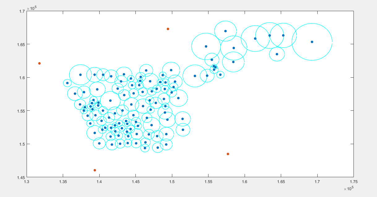
绘图结果:
figure1:
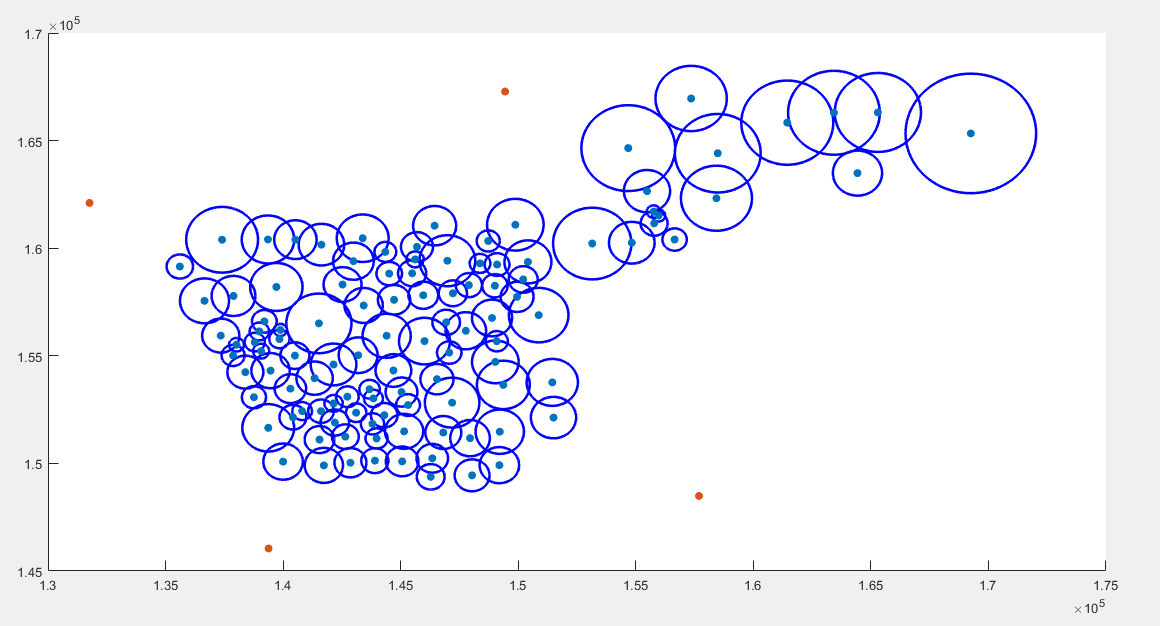
figure2:
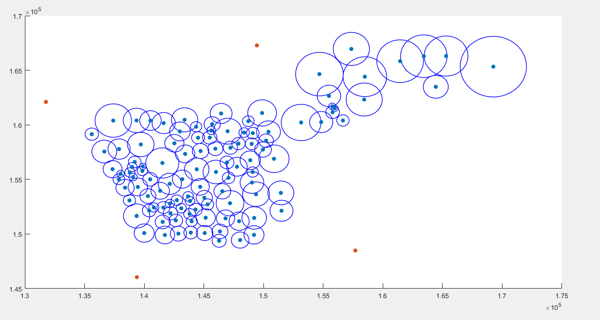
figure3:
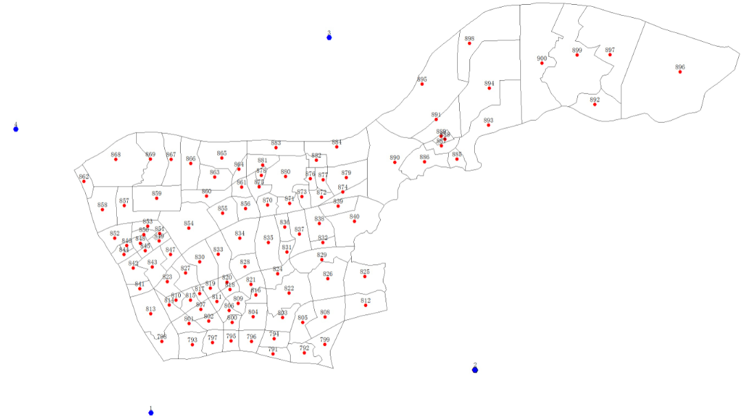
赛题具体地图:
参考资料:
1.https://blog.csdn.net/ZLK961543260/article/details/70216089
2.数据来源为2017年研究生数学建模竞赛F题赛题数据