逻辑回归
1、 总述
逻辑回归来源于回归分析,用来解决分类问题,即预测值变为较少数量的离散值。
2、 基本概念
回归分析(Regression Analysis):存在一堆观测资料,希望获得数据内在分布规律。单个样本表示成二维或多维向量,包含一个因变量Y和一个或多个自变量X。回归分析主要研究当自变量变化时,因变量如何变化,数学表示成Y=f(X),其中函数f称为回归函数(regression function)。回归分析最终目的是找到最能代表已观测数据的回归函数。
分类:因变量Y为有限离散集,即y∈{1,2,3…}。利用训练得到的回归模型hθ(x)进行分类,设定阈值0.5。如果hθ(x)>=0.5,预测结果为“y=1”,相反hθ(x)<0.5,预测结果为“y=0”。这里hθ(x)的值可以>1 或<0。对于逻辑回归分类来说,希望0<=hθ(x)<=1。
逻辑函数:也成为Sigmoid函数。线性回归中hθ(x)=θTx,显然无法限定输出到0,1之间。所以逻辑回归的Hypothesis表示为:hθ(x)=g(θTx)。这里g称为Sigmoid函数,表达式为:g(z)=1/(1+e-z),图形如下:
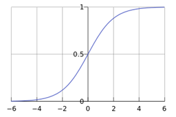
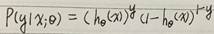
于是逻辑回归的Hypothesis最终表示为hθ(x)=1/(1+e-θTx),含义是给定输入x,参数化的θ(参数空间),输出y=1的概率。也可表示为
hθ(x)=P(y=1|x;θ) (1)
对于二分类问题,P(y=1|x;θ)+ P(y=0|x;θ)=1,所以
P(y=0|x;θ)=1- P(y=1|x;θ) (2)
决策边界(Decision boundary):对于hθ(x)同样设定阈值0.5,当hθ(x)>=0.5时,y=1,此时θTx>=0。当hθ(x)<0.5时,y=0,此时θTx<0。所以可以认为θTx=0是一个决策边界。
代价函数(Cost function):线性回归代价函数定义为:
可以简写为:
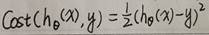
上述代价函数为凸函数,对于凸函数来说局部最小值即为全局最小值,所以只要求得一个局部极小值,该点一定为全局极小值点。将逻辑回归hθ(x)=1/(1+e-θTx)代入上面的代价函数,会存在问题即函数“非凸”的,所以需要引入其它代价函数。
逻辑回归代价函数定义为:
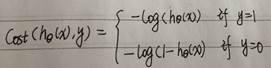
当y=1时,函数曲线如下:
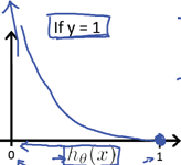
当y=1,hθ(x)=1时,cost为0,也就是预测值与真实值完全相等时,代价为0.当hθ(x)->0时,cost->∞。当hθ(x)=0,也就是P(y=1|x;θ)=0,也就是预测y=1的概率为0,此时惩罚cost值趋向无穷大。
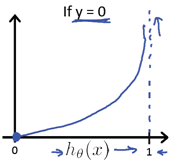
同样的,y=0情况类似。
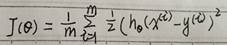
简化代价函数及梯度下降求解:逻辑回归的代价函数可以简写为:
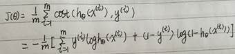
中括号中式子为对逻辑回归函数进行最大似然估计求解的最大似然函数,对最大似然函数求最大值,从而得到参数θ的估计。具体推导留到下节。这里类似,求解代价函数取的最小值时的参数θ。含义不同,实际上公示一样。与线性回归类似,可以利用梯度下降法求解参数θ。
优化求解算法:共轭梯度(Conjugate gradient)、BFGS、L-BFGS算法。优点是不需要人工挑选学习步长α,通常速度比梯度下降法快。缺点通常更复杂。
3、 算法求解
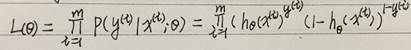
最大似然估计求解:综合式(1)和式(2)得到概率函数为:
似然函数为:
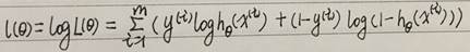
对数似然函数为:
可以看出代价函数J(θ)=-l(θ)/m。利用梯度上升法求对数似然函数取最大值的参数θ,等价于梯度下降法求代价函数J取最小值时的参数θ。
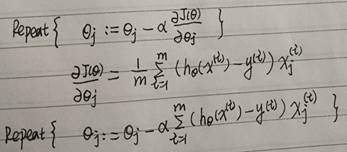
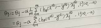
梯度下降法求解:
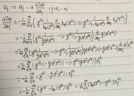
其中,用到了下面的求导公示:
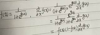
最终结果为:
4、 附录
代价函数:监督学习问题是在假设空间F中选取模型f作为决策函数,对于给定的输入X,由f(X)给出相应的输出Y,这个输出的预测值f(X)与真实Y可能不一致。用一个损失函数(loss function)或代价函数(cost function)来度量预测错误的程度。损失函数是f(x)和Y的非负实值函数,记做L(Y, f(X))。
5、附
逻辑回归--theano
"""
This tutorial introduces logistic regression using Theano and stochastic
gradient descent.

Logistic regression is a probabilistic, linear classifier. It is parametrized
by a weight matrix :math:`W` and a bias vector :math:`b`. Classification is
done by projecting data points onto a set of hyperplanes, the distance to
which is used to determine a class membership probability.

Mathematically, this can be written as:

.. math::
  P(Y=i|x, W,b) &= softmax_i(W x + b) \
                &= frac {e^{W_i x + b_i}} {sum_j e^{W_j x + b_j}}


The output of the model or prediction is then done by taking the argmax of
the vector whose i'th element is P(Y=i|x).

.. math::

  y_{pred} = argmax_i P(Y=i|x,W,b)


This tutorial presents a stochastic gradient descent optimization method
suitable for large datasets.


References:

    - textbooks: "Pattern Recognition and Machine Learning" -
                 Christopher M. Bishop, section 4.3.2

"""
from __future__ import print_function

__docformat__ = 'restructedtext en'

import six.moves.cPickle as pickle
import gzip
import os
import sys
import timeit
import numpy
import theano
import theano.tensor as T

class LogisticRegression(object):
    """Multi-class Logistic Regression Class

    The logistic regression is fully described by a weight matrix :math:`W`
    and bias vector :math:`b`. Classification is done by projecting data
    points onto a set of hyperplanes, the distance to which is used to
    determine a class membership probability.
    """

    def __init__(self, input, n_in, n_out):
        """ Initialize the parameters of the logistic regression

        :type input: theano.tensor.TensorType
        :param input: symbolic variable that describes the input of the
                      architecture (one minibatch)

        :type n_in: int
        :param n_in: number of input units, the dimension of the space in
                     which the datapoints lie

        :type n_out: int
        :param n_out: number of output units, the dimension of the space in
                      which the labels lie

        """
        # start-snippet-1
        # initialize with 0 the weights W as a matrix of shape (n_in, n_out)
        self.W = theano.shared(
            value=numpy.zeros(
                (n_in, n_out),#n_in = 784,图片数据点,n_out = 10 输出类别数
                dtype=theano.config.floatX
            ),
            name='W',#变量名
            borrow=True#使用共享变量
        )
        # initialize the biases b as a vector of n_out 0s
        #b是偏倚项向量,初始值都是0,这里没写成向量是因为之后要广播形式。
        self.b = theano.shared(
            value=numpy.zeros(
                (n_out,),
                dtype=theano.config.floatX
            ),
            name='b',
            borrow=True
        )

        # symbolic expression for computing the matrix of class-membership
        # probabilities
        # Where:
        # W is a matrix where column-k represent the separation hyperplane for
        # class-k
        # x is a matrix where row-j  represents input training sample-j
        # b is a vector where element-k represent the free parameter of
        # hyperplane-k
        self.p_y_given_x = T.nnet.softmax(T.dot(input, self.W) + self.b)#nnet里面封装机器学习算法

        # symbolic description of how to compute prediction as class whose
        # probability is maximal
        self.y_pred = T.argmax(self.p_y_given_x, axis=1)#argmax返回最大值下标,因为本例数据集是MNIST,下标刚好就是类别。axis=1表示按行操作。
        # end-snippet-1

        # parameters of the model
        self.params = [self.W, self.b]

        # keep track of model input
        self.input = input

    def negative_log_likelihood(self, y):
        """Return the mean of the negative log-likelihood of the prediction
        of this model under a given target distribution.

        .. math::

            frac{1}{|mathcal{D}|} mathcal{L} (	heta={W,b}, mathcal{D}) =
            frac{1}{|mathcal{D}|} sum_{i=0}^{|mathcal{D}|}
                log(P(Y=y^{(i)}|x^{(i)}, W,b)) \
            ell (	heta={W,b}, mathcal{D})

        :type y: theano.tensor.TensorType
        :param y: corresponds to a vector that gives for each example the
                  correct label

        Note: we use the mean instead of the sum so that
              the learning rate is less dependent on the batch size
        """
        # start-snippet-2
        # y.shape[0] is (symbolically) the number of rows in y, i.e.,
        # number of examples (call it n) in the minibatch
        # T.arange(y.shape[0]) is a symbolic vector which will contain
        # [0,1,2,... n-1] T.log(self.p_y_given_x) is a matrix of
        # Log-Probabilities (call it LP) with one row per example and
        # one column per class LP[T.arange(y.shape[0]),y] is a vector
        # v containing [LP[0,y[0]], LP[1,y[1]], LP[2,y[2]], ...,
        # LP[n-1,y[n-1]]] and T.mean(LP[T.arange(y.shape[0]),y]) is
        # the mean (across minibatch examples) of the elements in v,
        # i.e., the mean log-likelihood across the minibatch.

        #代价函数NLL
        #因为我们是MSGD,每次训练一个batch,一个batch有n_example个样本,则y大小是(n_example,),
        #y.shape[0]得出行数即样本数,将T.log(self.p_y_given_x)简记为LP,LP是样本数个行,10列;每行的10个数为对应10个类别的10个概率
        #则LP[T.arange(y.shape[0]),y]得到[LP[0,y[0]], LP[1,y[1]], LP[2,y[2]], ...,LP[n-1,y[n-1]]]。LP[n-1,y[n-1]]为第n-1行第n-1列,是第n-1个样本所对应10个类别中一个类别的概率
        #最后求均值mean,也就是说,minibatch的SGD,是计算出batch里所有样本的NLL的平均值,作为它的cost
        return -T.mean(T.log(self.p_y_given_x)[T.arange(y.shape[0]), y])
        # end-snippet-2

    def errors(self, y):
        """Return a float representing the number of errors in the minibatch
        over the total number of examples of the minibatch ; zero one
        loss over the size of the minibatch

        :type y: theano.tensor.TensorType
        :param y: corresponds to a vector that gives for each example the
                  correct label
        """

        # check if y has same dimension of y_pred。# 首先检查y与y_pred的维度是否一样,即是否含有相等的样本数
        if y.ndim != self.y_pred.ndim:
            raise TypeError(
                'y should have the same shape as self.y_pred',
                ('y', y.type, 'y_pred', self.y_pred.type)
            )
        # check if y is of the correct datatype
        if y.dtype.startswith('int'):
            # the T.neq operator returns a vector of 0s and 1s, where 1
            # represents a mistake in prediction
            # 再检查是不是int类型,是的话计算T.neq(self.y_pred, y)的均值,作为误差率
            #举个例子,假如self.y_pred=[3,2,3,2,3,2],而实际上y=[3,4,3,4,3,4]
            #则T.neq(self.y_pred, y)=[0,1,0,1,0,1],1表示不等,0表示相等
            #故T.mean(T.neq(self.y_pred, y))=T.mean([0,1,0,1,0,1])=0.5,即错误率50%
            return T.mean(T.neq(self.y_pred, y))
        else:
            raise NotImplementedError()


def load_data(dataset):
    ''' Loads the dataset

    :type dataset: string
    :param dataset: the path to the dataset (here MNIST)
    '''

    #############
    # LOAD DATA #
    #############

    # Download the MNIST dataset if it is not present
    data_dir, data_file = os.path.split(dataset)
    if data_dir == "" and not os.path.isfile(dataset):
        # Check if dataset is in the data directory.
        new_path = os.path.join(#连接两个文件名的地址
            os.path.split(__file__)[0],#当前脚本的路径
            "..",
            "data",
            dataset
        )
        if os.path.isfile(new_path) or data_file == 'mnist.pkl.gz':
            dataset = new_path

    if (not os.path.isfile(dataset)) and data_file == 'mnist.pkl.gz':
        from six.moves import urllib
        origin = (
            'http://www.iro.umontreal.ca/~lisa/deep/data/mnist/mnist.pkl.gz'
        )
        print('Downloading data from %s' % origin)
        urllib.request.urlretrieve(origin, dataset)

    print('... loading data')

    # Load the dataset
    with gzip.open(dataset, 'rb') as f:
        try:
            train_set, valid_set, test_set = pickle.load(f, encoding='latin1')
        except:
            train_set, valid_set, test_set = pickle.load(f)
    # train_set, valid_set, test_set format: tuple(input, target)
    # input is a numpy.ndarray of 2 dimensions (a matrix)
    # where each row corresponds to an example. target is a
    # numpy.ndarray of 1 dimension (vector) that has the same length as
    # the number of rows in the input. It should give the target
    # to the example with the same index in the input.

    #将数据设置成shared variables,主要时为了GPU加速,只有shared variables才能存到GPU memory中
    #GPU里数据类型只能是float。而data_y是类别,所以最后又转换为int返回
    def shared_dataset(data_xy, borrow=True):
        """ Function that loads the dataset into shared variables

        The reason we store our dataset in shared variables is to allow
        Theano to copy it into the GPU memory (when code is run on GPU).
        Since copying data into the GPU is slow, copying a minibatch everytime
        is needed (the default behaviour if the data is not in a shared
        variable) would lead to a large decrease in performance.
        """
        data_x, data_y = data_xy
        shared_x = theano.shared(numpy.asarray(data_x,#asrray将输入的数据转化为矩阵的形式
                                               dtype=theano.config.floatX),
                                 borrow=borrow)
        shared_y = theano.shared(numpy.asarray(data_y,
                                               dtype=theano.config.floatX),
                                 borrow=borrow)
        # When storing data on the GPU it has to be stored as floats
        # therefore we will store the labels as ``floatX`` as well
        # (``shared_y`` does exactly that). But during our computations
        # we need them as ints (we use labels as index, and if they are
        # floats it doesn't make sense) therefore instead of returning
        # ``shared_y`` we will have to cast it to int. This little hack
        # lets ous get around this issue
        return shared_x, T.cast(shared_y, 'int32')#cast数据类型转换

    test_set_x, test_set_y = shared_dataset(test_set)
    valid_set_x, valid_set_y = shared_dataset(valid_set)
    train_set_x, train_set_y = shared_dataset(train_set)

    rval = [(train_set_x, train_set_y), (valid_set_x, valid_set_y),
            (test_set_x, test_set_y)]
    return rval


def sgd_optimization_mnist(learning_rate=0.13, n_epochs=1000,
                           dataset='mnist.pkl.gz',
                           batch_size=600):
    """
    Demonstrate stochastic gradient descent optimization of a log-linear
    model

    This is demonstrated on MNIST.

    :type learning_rate: float
    :param learning_rate: learning rate used (factor for the stochastic
                          gradient)

    :type n_epochs: int
    :param n_epochs: maximal number of epochs to run the optimizer

    :type dataset: string
    :param dataset: the path of the MNIST dataset file from
                 http://www.iro.umontreal.ca/~lisa/deep/data/mnist/mnist.pkl.gz

    """
    datasets = load_data(dataset)

    train_set_x, train_set_y = datasets[0]
    valid_set_x, valid_set_y = datasets[1]
    test_set_x, test_set_y = datasets[2]

    # compute number of minibatches for training, validation and testing
    #计算有多少个minibatch,因为我们的优化算法是MSGD,是一个batch一个batch来计算cost的
    n_train_batches = train_set_x.get_value(borrow=True).shape[0] // batch_size
    n_valid_batches = valid_set_x.get_value(borrow=True).shape[0] // batch_size
    n_test_batches = test_set_x.get_value(borrow=True).shape[0] // batch_size

    ######################
    # BUILD ACTUAL MODEL #
    ######################
    print('... building the model')

    # allocate symbolic variables for the data
    #设置变量,index表示minibatch的下标,x表示训练样本,y是对应的label
    index = T.lscalar()  # index to a [mini]batch

    # generate symbolic variables for input (x and y represent a
    # minibatch)
    x = T.matrix('x')  # data, presented as rasterized images
    y = T.ivector('y')  # labels, presented as 1D vector of [int] labels

    # construct the logistic regression class
    # Each MNIST image has size 28*28
    classifier = LogisticRegression(input = x, n_in = 28*28, n_out = 10)

    # the cost we minimize during training is the negative log likelihood of
    # the model in symbolic format
    #定义代价函数,用y来初始化代价函数,而其实还有一个隐含的参数x在classifier中。
    #这样理解才是合理的,因为cost必须由x和y得来,单单y是得不到cost的。
    cost = classifier.negative_log_likelihood(y)

    # compiling a Theano function that computes the mistakes that are made by
    # the model on a minibatch
    #这里必须说明一下theano的function函数,givens是字典,其中的x、y是key,冒号后面是它们的value。
    #在function被调用时,x、y将被具体地替换为它们的value,而value里的参数index就是inputs=[index]这里给出。
    #下面举个例子:
    #比如test_model(1),首先根据index=1具体化x为test_set_x[1 * batch_size: (1 + 1) * batch_size],
    #具体化y为test_set_y[1 * batch_size: (1 + 1) * batch_size]。然后函数计算outputs=classifier.errors(y),
    #这里面有参数y和隐含的x,所以就将givens里面具体化的x、y传递进去。
    test_model = theano.function(
        inputs=[index],
        outputs=classifier.errors(y),#错误率
        givens={
            x: test_set_x[index * batch_size: (index + 1) * batch_size],
            y: test_set_y[index * batch_size: (index + 1) * batch_size]
        }
    )

    validate_model = theano.function(
        inputs=[index],
        outputs=classifier.errors(y),
        givens={
            x: valid_set_x[index * batch_size: (index + 1) * batch_size],
            y: valid_set_y[index * batch_size: (index + 1) * batch_size]
        }
    )

    # compute the gradient of cost with respect to theta = (W,b)
    g_W = T.grad(cost=cost, wrt=classifier.W)
    g_b = T.grad(cost=cost, wrt=classifier.b)

    # start-snippet-3
    # specify how to update the parameters of the model as a list of
    # (variable, update expression) pairs.
    updates = [(classifier.W, classifier.W - learning_rate * g_W),
               (classifier.b, classifier.b - learning_rate * g_b)]

    # compiling a Theano function `train_model` that returns the cost, but in
    # the same time updates the parameter of the model based on the rules
    # defined in `updates`
    train_model = theano.function(#这里是这样运行的,先是index变了,然后x,y变了,然后cost变了,然后g_w变了,然后updates变了
        inputs=[index],
        outputs=cost,
        updates=updates,#这里的update参数更新了shared变量
        givens={
            x: train_set_x[index * batch_size: (index + 1) * batch_size],
            y: train_set_y[index * batch_size: (index + 1) * batch_size]
        }
    )
    # end-snippet-3

    ###############
    # TRAIN MODEL #
    ###############
    print('... training the model')
    # early-stopping parameters
    patience = 5000  # look as this many examples regardless
    patience_increase = 2  # wait this much longer when a new best is found

    #提高的阈值,在验证误差减小到之前的0.995倍时,会更新best_validation_loss
    improvement_threshold = 0.995  # a relative improvement of this much is
                                  # considered significant
    #这样设置validation_frequency可以保证每一次epoch都会在验证集上测试
    validation_frequency = min(n_train_batches, patience // 2)#//地板除
                                  # go through this many
                                  # minibatche before checking the network
                                  # on the validation set; in this case we
                                  # check every epoch

    best_validation_loss = numpy.inf#最好的验证集上的loss,最好即最小。初始化为无穷大
    test_score = 0.
    start_time = timeit.default_timer()

    done_looping = False
    epoch = 0
    #下面就是训练过程了,while循环控制的时步数epoch,一个epoch会遍历所有的batch,即所有的图片。
    #for循环是遍历一个个batch,一次一个batch地训练。for循环体里会用train_model(minibatch_index)去训练模型,
    #train_model里面的updatas会更新各个参数。
    #for循环里面会累加训练过的batch数iter,当iter是validation_frequency倍数时则会在验证集上测试,
    #如果验证集的损失this_validation_loss小于之前最佳的损失best_validation_loss,
    #则更新best_validation_loss和best_iter,同时在testset上测试。
    #如果验证集的损失this_validation_loss小于best_validation_loss*improvement_threshold时则更新patience。
    #当达到最大步数n_epoch时,或者patience<iter时,结束训练
    while (epoch < n_epochs) and (not done_looping):
        epoch = epoch + 1
        print('epoch',epoch)
        for minibatch_index in range(n_train_batches):#n_train_batches训练语料的批次数,一个for循环一个批次

            minibatch_avg_cost = train_model(minibatch_index)#一个批次的代价
            # iteration number
            iter = (epoch - 1) * n_train_batches + minibatch_index
            if (iter + 1) % validation_frequency == 0:
                # compute zero-one loss on validation set
                validation_losses = [validate_model(i)
                                     for i in range(n_valid_batches)]
                this_validation_loss = numpy.mean(validation_losses)

                print(
                    'epoch %i, minibatch %i/%i, validation error %f %%' %
                    (
                        epoch,
                        minibatch_index + 1,
                        n_train_batches,
                        this_validation_loss * 100.
                    )
                )

                # if we got the best validation score until now
                if this_validation_loss < best_validation_loss:
                    #improve patience if loss improvement is good enough
                    if this_validation_loss < best_validation_loss *
                       improvement_threshold:
                        patience = max(patience, iter * patience_increase)

                    best_validation_loss = this_validation_loss
                    # test it on the test set

                    test_losses = [test_model(i)
                                   for i in range(n_test_batches)]
                    test_score = numpy.mean(test_losses)

                    print(
                        (
                            '     epoch %i, minibatch %i/%i, test error of'
                            ' best model %f %%'
                        ) %
                        (
                            epoch,
                            minibatch_index + 1,
                            n_train_batches,
                            test_score * 100.
                        )
                    )

                    # save the best model
                    with open('best_model.pkl', 'wb') as f:
                        pickle.dump(classifier, f)

            if patience <= iter:
                done_looping = True
                break

    end_time = timeit.default_timer()
    print(
        (
            'Optimization complete with best validation score of %f %%,'
            'with test performance %f %%'
        )
        % (best_validation_loss * 100., test_score * 100.)
    )
    print('The code run for %d epochs, with %f epochs/sec' % (
        epoch, 1. * epoch / (end_time - start_time)))
    print(('The code for file ' +
           os.path.split(__file__)[1] +
           ' ran for %.1fs' % ((end_time - start_time))), file=sys.stderr)


def predict():
    """
    An example of how to load a trained model and use it
    to predict labels.
    """

    # load the saved model
    classifier = pickle.load(open('best_model.pkl'))

    # compile a predictor function
    predict_model = theano.function(
        inputs=[classifier.input],
        outputs=classifier.y_pred)

    # We can test it on some examples from test test
    dataset='mnist.pkl.gz'
    datasets = load_data(dataset)
    test_set_x, test_set_y = datasets[2]
    test_set_x = test_set_x.get_value()

    predicted_values = predict_model(test_set_x[:10])
    print("Predicted values for the first 10 examples in test set:")
    print(predicted_values)


if __name__ == '__main__':
    sgd_optimization_mnist()
参考
http://ilanever.com/article/detail.do;jsessionid=9A6E0C3D33ECADD6723113777AA6DE9C?id=260
http://52opencourse.com/125/coursera公开课笔记-斯坦福大学机器学习第六课-逻辑回归-logistic-regression
李航:《统计学习方法》
http://blog.csdn.net/dongtingzhizi/article/details/15962797
http://blog.jasonding.top/2015/01/09/Machine%20Learning/【机器学习基础】Logistic回归基础
http://www.cnblogs.com/jerrylead/archive/2011/03/05/1971867.html