决策树算法小结(三) CART原理及代码实现

前面总结了决策树ID3算法(ID3原理及代码实现)和改进版C4.5算法(C4.5原理及代码实现)，它们存在一些不如，如只能处理分类不能处理回归存在过拟合等问题。因此，有必要介绍一个新的叫做CART（Classification And Regression Trees，分类回归树）的树构建算法。该算法既可以用于分类还可以用于回归，它使用二元切分来处理连续型变量。
决策树算法三要素：特征选择 决策树生成 决策树减枝

1 CART原理

CART算法有两步：
- 决策树生成：基于训练数据集生成决策树，生成的决策树要尽量大;
- 决策树剪枝：用验证数据集对已生成的树进行剪枝并选择最优子树，这时用损失函数最小作为剪枝的标准。(树剪枝主要目的是降低决策树的复杂度来避免过拟合)

1.1 CART分类树算法——特征选择

分类树用基尼指数选择最优特征，同时决定该特征的最优二值切分点
基尼指数
分类问题中，假设有(K)个类，样本点属于第(k)类的概率为(p_{k})，则概率分布的基尼指数表达式：

[Gini(p)=sum_{k=1}^{K}p_{k}(1-p_{k})=1-sum_{k=1}^{K}p_{k}^{2} ]

二分类中，若样本点属于第一个类的概率是(p)，则概率分布的基尼指数表达式：

[Gini(p)=2p(1-p) ]

对于给定的样本集合(D)，基尼指数表达式：

[Gini(D)=1-sum_{k=1}^{K}left ( frac{|C_{k}|}{|D|} ight )^{2} ]

其中(K)表示类的个数，(C_{k})是样本集合(D)中属于第(k)类的样本子集，(|C_{k}|)表示第(k)个类别的个数。

1.2 CART分类树生成算法

输入：训练数据集(D)，停止计算的条件;

输出：CART决策树
根据训练数据集，从根节点开始，递归地构建二叉决策树

step1 对于当前节点的数据集为(D)，如果样本个数小于阈值或者没有特征，则返回决策子树，当前节点停止递归;

step2 计算样本集(D)的基尼系数，如果基尼系数小于阈值，则返回决策树子树，当前节点停止递归;

step3 计算当前节点现有的各个特征的各个特征值对数据集D的基尼系数;

step4 在计算出来的各个特征的各个特征值对数据集(D)的基尼系数中，选择基尼系数最小的特征(A)和对应的特征值(a)。根据这个最优特征和最优特征值，把数据集划分成两部分(D1)和4D2￥，同时建立当前节点的左右节点，做节点的数据集(D)为(D1)，右节点的数据集(D)为(D2);

step5 对左右的子节点递归的调用1-4步，生成决策树.

算法停止计算的条件是结点中的样本个数小于预定阈值，或样本集的基尼指数小于预测阈值(样本基本属于同一类)，或者更多特征。

1.3 CART回归树生成算法

决策树的生成就是递归地构建二叉决策树的过程，对回归树用平方误差最小化准则，对分类树用基尼指数(Gini index)最小化准则，进行特征选择，生成二叉树。

最小二乘回归树生成算法
CART回归树的度量目标是，对于任意划分特征(A)，对应的任意划分点s两边划分成的数据集(D1)和(D2)，求出使(D14和)D2(各自集合的均方差最小，同时)D1(和)D24的均方差之和最小所对应的特征和特征值划分点。表达式为：

[min_{A,s}left [ min_{c_{1}} sum_{x_{i}epsilon D_{1}(A,s)}(y_{i}-c_{1})^{2}+min_{c_{2}}sum_{x_{i}epsilon D_{2}(A,s)}(y_{i}-c_{2})^{2} ight ] ]

其中，(c_{1})表示(D_{1})数据集的样本输出均值，(c_{2})表示(D_{2})数据集的样本输出均值。

1.4 CART剪枝

CART回归树和CART分类树的剪枝策略除了在度量损失的时候一个使用均方差，一个使用基尼系数，算法基本完全一样

CART剪枝算法
输入 CART算法生成的决策树(T_{0});

输出 最优决策树(T_{alpha }).

step1 设(k=0)，(T=T_{0}).

step2 设$alpha = +infty $.

step3 自下而上地对各内部结点(t)计算(C(T_{t}))，(|T_{t}|)和(g(t)=frac{C(t)-C(T_{t})}{|T_{t}|-1}) (alpha =min(alpha ,g(t)))，其中，(T_{t})表示以t为根结点的子树，(C(T_{t}))是对训练数据的预测误差，(|T_{t}|)是(T_{t})的叶结点个数.

step4 自上而下地访问内部结点(t)，若(g(t)=alpha)，进行剪枝，并对叶结点(t)以多数表决法决定其类，得到树(T).

step5 设(k=k+1)，(alpha _{k}=alpha)，(T_{k}=T).

step6 如果(T)不是由根结点单独构成的树，则回到步骤(4).

step7 采用交叉验证法在子树序列(T_{0},T_{1},cdots ,T_{n})中选取最优树(T_{alpha})

2 CART分类树代码实现

3 CART回归树代码实现

CART回归算法递归构建树

from numpy import *
def loadDataSet(fileName):

dataMat = []

fr = open(fileName)

for line in fr.readlines():

curLine = line.strip().split('	')

fltLine = list(map(float,curLine)) #将每行映射成浮点数

dataMat.append(fltLine)

return dataMat
def binSplitDataSet(dataSet,feature,value):  #通过数组过滤方式将数据集切分得到两个子集返回

"""
:param dataSet: 数据集
:param feature: 待切分的特征
:param value: 特征对应的值
:return:
"""
mat0 = dataSet[nonzero(dataSet[:,feature] > value)[0],:]
mat1 = dataSet[nonzero(dataSet[:,feature] <= value)[0], :]
return mat0,mat1

def createTree(dataSet, leafType=regLeaf, errType=regErr, ops=(1,4)): #递归函数 树构建

"""
:param dataSet: 数据集
:param leafType: 对创建叶节点的函数的引用
:param errType: 对误差计算函数的引用
:param ops: 用于树构建所需其他参数的元组
:return:
"""
feat, val = chooseBestSplit(dataSet, leafType, errType, ops)
if feat == None: return val   #满足停止条件时返回叶节点值
retTree = {}
retTree['spInd'] = feat
retTree['spVal'] = val
lSet, rSet = binSplitDataSet(dataSet, feat, val)
retTree['left'] = createTree(lSet, leafType, errType, ops)
retTree['right'] = createTree(rSet, leafType, errType, ops)
return retTree

将CART 算法用于回归

回归树的切分函数

def regLeaf(dataSet):
    return mean(dataSet[:,-1])
def regErr(dataSet):

return var(dataSet[:,-1])*shape(dataSet)[0]
def chooseBestSplit(dataSet, leafType=regLeaf, errType=regErr, ops=(1,4)): #用最佳方式切分数据集 生成相应的叶节点

tolS = ops[0]; tolN = ops[1]

#if all the target variables are the same value: quit and return value

if len(set(dataSet[:,-1].T.tolist()[0])) == 1: #exit cond 1

return None, leafType(dataSet)

m,n = shape(dataSet)

#the choice of the best feature is driven by Reduction in RSS error from mean

S = errType(dataSet)

bestS = inf; bestIndex = 0; bestValue = 0

for featIndex in range(n-1):

for splitVal in set((dataSet[:,featIndex].T.A.tolist())[0]):

mat0, mat1 = binSplitDataSet(dataSet, featIndex, splitVal)

if (shape(mat0)[0] < tolN) or (shape(mat1)[0] < tolN): continue

newS = errType(mat0) + errType(mat1)

if newS < bestS:

bestIndex = featIndex

bestValue = splitVal

bestS = newS

#if the decrease (S-bestS) is less than a threshold don't do the split

if (S - bestS) < tolS:

return None, leafType(dataSet) #exit cond 2

mat0, mat1 = binSplitDataSet(dataSet, bestIndex, bestValue)

if (shape(mat0)[0] < tolN) or (shape(mat1)[0] < tolN):  #exit cond 3

return None, leafType(dataSet)

return bestIndex,bestValue#returns the best feature to split on

#and the value used for that split

控制台运行效果:

>>> import regTrees
>>> import imp
>>> imp.reload(regTrees)
<module 'regTrees' from 'D:\Python\Mechine_learning\RegTree\regTrees.py'>
>>> testMat=mat(eye(4))
>>> mat0,mat1=regTrees.binSplitDataSet(testMat,1,0.5)
>>> mat0
matrix([[0., 1., 0., 0.]])
>>> mat1
matrix([[1., 0., 0., 0.],
        [0., 0., 1., 0.],
        [0., 0., 0., 1.]])

>>> imp.reload(regTrees)
<module 'regTrees' from 'D:\Python\Mechine_learning\RegTree\regTrees.py'>
>>> from numpy import *
>>> myDat=regTrees.loadDataSet('ex00.txt')
>>> myMat=mat(myDat)
>>> regTrees.createTree(myMat)
{'spInd': 0, 'spVal': 0.48813, 'left': 1.0180967672413792, 'right': -0.04465028571428572}
>>> import matplotlib.pyplot as plt
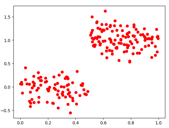
>>> plt.plot(myMat[:,0],myMat[:,1],'ro')
[<matplotlib.lines.Line2D object at 0x000002105E508A20>]
>>> plt.show()

>>> myDat1=regTrees.loadDataSet('ex0.txt')
>>> myMat1=mat(myDat1)
>>> regTrees.createTree(myMat1)
{'spInd': 1, 'spVal': 0.39435, 'left': {'spInd': 1, 'spVal': 0.582002, 'left': {'spInd': 1, 'spVal': 0.797583, 'left': 3.9871632, 'right': 2.9836209534883724}, 'right': 1.980035071428571}, 'right': {'spInd': 1, 'spVal': 0.197834, 'left': 1.0289583666666666, 'right': -0.023838155555555553}}
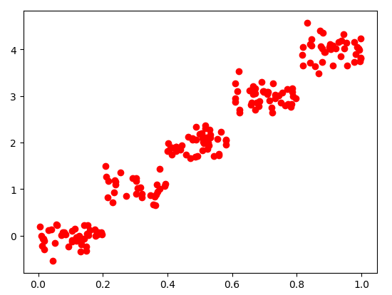
>>> plt.plot(myMat1[:,1],myMat1[:,2],'ro')
[<matplotlib.lines.Line2D object at 0x000002105DCD54E0>]
>>> plt.show()

ex00.txt切分后的数据点：

ex0.txt切分后的数据点：

3.1 预剪枝

用数据来构建一棵新的树（数据存放在ex2.txt中）,观察y轴就会发现，这里的数量级是ex00.txt构建树的100倍，且这里构建的新树则有很多叶节点。产生这个现象的原因在于，停止条件tolS对误差的数量级十分敏感。如果在选项中花费时间并对上述误差容忍度取平方值，或许也能得到仅有两个叶节点组成的树

预剪枝

>>> myDat2=regTrees.loadDataSet('ex2.txt')
>>> myMat2=mat(myDat2)
>>> regTrees.createTree(myMat2)
{'spInd': 0, 'spVal': 0.499171, 'left': {'spInd': 0, 'spVal': 0.729397, 'left': {'spInd': 0, 'spVal': 0.952833, 'left': {'spInd': 0, 'spVal': 0.958512, 'left': 105.24862350000001, 'right': 112.42895575000001}, 'right': {'spInd': 0, 'spVal': 0.759504, 'left': {'spInd': 0, 'spVal': 0.790312, 'left': {'spInd': 0, 'spVal': 0.833026, 'left': {'spInd': 0, 'spVal': 0.944221, 'left': 87.3103875, 'right': {'spInd': 0, 'spVal': 0.85497, 'left': {'spInd': 0, 'spVal': 0.910975, 'left': 96.452867, 'right': {'spInd': 0, 'spVal': 0.892999, 'left': 104.825409, 'right': {'spInd': 0, 'spVal': 0.872883, 'left': 95.181793, 'right': 102.25234449999999}}}, 'right': 95.27584316666666}}, 'right': {'spInd': 0, 'spVal': 0.811602, 'left': 81.110152, 'right': 88.78449880000001}}, 'right': 102.35780185714285}, 'right': 78.08564325}}, 'right': {'spInd': 0, 'spVal': 0.640515, 'left': {'spInd': 0, 'spVal': 0.666452, 'left': {'spInd': 0, 'spVal': 0.706961, 'left': 114.554706, 'right': {'spInd': 0, 'spVal': 0.698472, 'left': 104.82495374999999, 'right': 108.92921799999999}}, 'right': 114.1516242857143}, 'right': {'spInd': 0, 'spVal': 0.613004, 'left': 93.67344971428572, 'right': {'spInd': 0, 'spVal': 0.582311, 'left': 123.2101316, 'right': {'spInd': 0, 'spVal': 0.553797, 'left': 97.20018024999999, 'right': {'spInd': 0, 'spVal': 0.51915, 'left': {'spInd': 0, 'spVal': 0.543843, 'left': 109.38961049999999, 'right': 110.979946}, 'right': 101.73699325000001}}}}}}, 'right': {'spInd': 0, 'spVal': 0.457563, 'left': {'spInd': 0, 'spVal': 0.467383, 'left': 12.50675925, 'right': 3.4331330000000007}, 'right': {'spInd': 0, 'spVal': 0.126833, 'left': {'spInd': 0, 'spVal': 0.373501, 'left': {'spInd': 0, 'spVal': 0.437652, 'left': -12.558604833333334, 'right': {'spInd': 0, 'spVal': 0.412516, 'left': 14.38417875, 'right': {'spInd': 0, 'spVal': 0.385021, 'left': -0.8923554999999995, 'right': 3.6584772500000016}}}, 'right': {'spInd': 0, 'spVal': 0.335182, 'left': {'spInd': 0, 'spVal': 0.350725, 'left': -15.08511175, 'right': -22.693879600000002}, 'right': {'spInd': 0, 'spVal': 0.324274, 'left': 15.05929075, 'right': {'spInd': 0, 'spVal': 0.297107, 'left': -19.9941552, 'right': {'spInd': 0, 'spVal': 0.166765, 'left': {'spInd': 0, 'spVal': 0.202161, 'left': {'spInd': 0, 'spVal': 0.217214, 'left': {'spInd': 0, 'spVal': 0.228473, 'left': {'spInd': 0, 'spVal': 0.25807, 'left': 0.40377471428571476, 'right': -13.070501}, 'right': 6.770429}, 'right': -11.822278500000001}, 'right': 3.4496025}, 'right': {'spInd': 0, 'spVal': 0.156067, 'left': -12.1079725, 'right': -6.247900000000001}}}}}}, 'right': {'spInd': 0, 'spVal': 0.084661, 'left': 6.509843285714284, 'right': {'spInd': 0, 'spVal': 0.044737, 'left': -2.544392714285715, 'right': 4.091626}}}}}
>>> import matplotlib.pyplot as plt
>>> plt.plot(myMat2[:,0],myMat2[:,1],'ro')
[]
>>> plt.show()

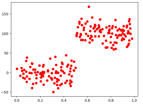
>>> regTrees.createTree(myMat2,ops=(10000,4))
{'spInd': 0, 'spVal': 0.499171, 'left': 101.35815937735848, 'right': -2.637719329787234}

其实，通过不断修改停止条件来得到合理结果并不是很好的办法。事实上，常常甚至不确定到底需要寻找什么样的结果。如果树节点过多，则该模型可能对数据过拟合，通过降低决策树的复杂度来避免过拟合的过程称为剪枝。在上面函数chooseBestSplit中的三个提前终止条件是“预剪枝”操作，另一种形式的剪枝需要使用测试集和训练集，称作“后剪枝”。
使用后剪枝方法需要将数据集交叉验证，首先给定参数，使得构建出的树足够复杂，之后从上而下找到叶节点，判断合并两个叶节点是否能够取得更好的测试误差，如果是就合并。

3.2 后剪枝

回归树剪枝函数

#判断输入是否为一棵树
def isTree(obj):
    return (type(obj).__name__=='dict') #判断为字典类型返回true
返回树的平均值
def getMean(tree):

if isTree(tree['right']):

tree['right'] = getMean(tree['right'])

if isTree(tree['left']):

tree['left'] = getMean(tree['left'])

return (tree['left']+tree['right'])/2.0
树的后剪枝
def prune(tree, testData):#待剪枝的树和剪枝所需的测试数据

if shape(testData)[0] == 0: return getMean(tree)  # 确认数据集非空

#假设发生过拟合，采用测试数据对树进行剪枝

if (isTree(tree['right']) or isTree(tree['left'])): #左右子树非空

lSet, rSet = binSplitDataSet(testData, tree['spInd'], tree['spVal'])

if isTree(tree['left']): tree['left'] = prune(tree['left'], lSet)

if isTree(tree['right']): tree['right'] = prune(tree['right'], rSet)

#剪枝后判断是否还是有子树

if not isTree(tree['left']) and not isTree(tree['right']):

lSet, rSet = binSplitDataSet(testData, tree['spInd'], tree['spVal'])

#判断是否merge

errorNoMerge = sum(power(lSet[:, -1] - tree['left'], 2)) + 

sum(power(rSet[:, -1] - tree['right'], 2))

treeMean = (tree['left'] + tree['right']) / 2.0

errorMerge = sum(power(testData[:, -1] - treeMean, 2))

#如果合并后误差变小

if errorMerge < errorNoMerge:

print("merging")

return treeMean

else:

return tree

else:

return tree

控制台运行效果

>>> imp.reload(regTrees)

>>> myTree=regTrees.createTree(myMat2, ops=(0,1))
>>> myDatTest=regTrees.loadDataSet('ex2test.txt')
>>> myMat2Test=mat(myDatTest)
>>> regTrees.prune(myTree, myMat2Test)
merging
merging
merging
merging
merging
merging
merging
merging
merging
merging
merging
merging
merging
merging
merging
merging
merging
merging
merging
merging
merging
merging
merging
merging
merging
merging
merging
merging
merging
merging
merging
merging
merging
merging
merging
merging
merging
merging
merging
merging
merging
merging
merging
merging
{'spInd': 0, 'spVal': 0.499171, 'left': {'spInd': 0, 'spVal': 0.729397, 'left': {'spInd': 0, 'spVal': 0.952833, 'left': {'spInd': 0, 'spVal': 0.965969, 'left': 92.5239915, 'right': {'spInd': 0, 'spVal': 0.956951, 'left': {'spInd': 0, 'spVal': 0.958512, 'left': {'spInd': 0, 'spVal': 0.960398, 'left': 112.386764, 'right': 123.559747}, 'right': 135.837013}, 'right': 111.2013225}}, 'right': {'spInd': 0, 'spVal': 0.759504, 'left': {'spInd': 0, 'spVal': 0.763328, 'left': {'spInd': 0, 'spVal': 0.769043, 'left': {'spInd': 0, 'spVal': 0.790312, 'left': {'spInd': 0, 'spVal': 0.806158, 'left': {'spInd': 0, 'spVal': 0.815215, 'left': {'spInd': 0, 'spVal': 0.833026, 'left': {'spInd': 0, 'spVal': 0.841547, 'left': {'spInd': 0, 'spVal': 0.841625, 'left': {'spInd': 0, 'spVal': 0.944221, 'left': {'spInd': 0, 'spVal': 0.948822, 'left': 96.41885225, 'right': 69.318649}, 'right': {'spInd': 0, 'spVal': 0.85497, 'left': {'spInd': 0, 'spVal': 0.936524, 'left': 110.03503850000001, 'right': {'spInd': 0, 'spVal': 0.934853, 'left': 65.548418, 'right': {'spInd': 0, 'spVal': 0.925782, 'left': 115.753994, 'right': {'spInd': 0, 'spVal': 0.910975, 'left': {'spInd': 0, 'spVal': 0.912161, 'left': 94.3961145, 'right': 85.005351}, 'right': {'spInd': 0, 'spVal': 0.901444, 'left': {'spInd': 0, 'spVal': 0.908629, 'left': 106.814667, 'right': 118.513475}, 'right': {'spInd': 0, 'spVal': 0.901421, 'left': 87.300625, 'right': {'spInd': 0, 'spVal': 0.892999, 'left': {'spInd': 0, 'spVal': 0.900699, 'left': 100.133819, 'right': 108.094934}, 'right': {'spInd': 0, 'spVal': 0.888426, 'left': 82.436686, 'right': {'spInd': 0, 'spVal': 0.872199, 'left': 98.54454949999999, 'right': 106.16859550000001}}}}}}}}}, 'right': {'spInd': 0, 'spVal': 0.84294, 'left': {'spInd': 0, 'spVal': 0.847219, 'left': 89.20993, 'right': 76.240984}, 'right': 95.893131}}}, 'right': 60.552308}, 'right': 124.87935300000001}, 'right': {'spInd': 0, 'spVal': 0.823848, 'left': 76.723835, 'right': {'spInd': 0, 'spVal': 0.819722, 'left': 59.342323, 'right': 70.054508}}}, 'right': {'spInd': 0, 'spVal': 0.811602, 'left': 118.319942, 'right': {'spInd': 0, 'spVal': 0.811363, 'left': 99.841379, 'right': 112.981216}}}, 'right': 73.49439925}, 'right': {'spInd': 0, 'spVal': 0.786865, 'left': 114.4008695, 'right': 102.26514075}}, 'right': 64.041941}, 'right': 115.199195}, 'right': 78.08564325}}, 'right': {'spInd': 0, 'spVal': 0.640515, 'left': {'spInd': 0, 'spVal': 0.642373, 'left': {'spInd': 0, 'spVal': 0.642707, 'left': {'spInd': 0, 'spVal': 0.665329, 'left': {'spInd': 0, 'spVal': 0.706961, 'left': {'spInd': 0, 'spVal': 0.70889, 'left': {'spInd': 0, 'spVal': 0.716211, 'left': 110.90283, 'right': {'spInd': 0, 'spVal': 0.710234, 'left': 103.345308, 'right': 108.553919}}, 'right': 135.416767}, 'right': {'spInd': 0, 'spVal': 0.698472, 'left': {'spInd': 0, 'spVal': 0.69892, 'left': {'spInd': 0, 'spVal': 0.699873, 'left': {'spInd': 0, 'spVal': 0.70639, 'left': 106.180427, 'right': 105.062147}, 'right': 115.586605}, 'right': 92.470636}, 'right': {'spInd': 0, 'spVal': 0.689099, 'left': 120.521925, 'right': {'spInd': 0, 'spVal': 0.666452, 'left': 101.91115275, 'right': 112.78136649999999}}}}, 'right': {'spInd': 0, 'spVal': 0.661073, 'left': 121.980607, 'right': {'spInd': 0, 'spVal': 0.652462, 'left': 115.687524, 'right': 112.715799}}}, 'right': 82.500766}, 'right': 140.613941}, 'right': {'spInd': 0, 'spVal': 0.613004, 'left': {'spInd': 0, 'spVal': 0.623909, 'left': {'spInd': 0, 'spVal': 0.628061, 'left': {'spInd': 0, 'spVal': 0.637999, 'left': 82.713621, 'right': {'spInd': 0, 'spVal': 0.632691, 'left': 91.656617, 'right': 93.645293}}, 'right': {'spInd': 0, 'spVal': 0.624827, 'left': 117.628346, 'right': 105.970743}}, 'right': 82.04976400000001}, 'right': {'spInd': 0, 'spVal': 0.606417, 'left': 168.180746, 'right': {'spInd': 0, 'spVal': 0.513332, 'left': {'spInd': 0, 'spVal': 0.533511, 'left': {'spInd': 0, 'spVal': 0.548539, 'left': {'spInd': 0, 'spVal': 0.553797, 'left': {'spInd': 0, 'spVal': 0.560301, 'left': {'spInd': 0, 'spVal': 0.599142, 'left': 93.521396, 'right': {'spInd': 0, 'spVal': 0.589806, 'left': 130.378529, 'right': {'spInd': 0, 'spVal': 0.582311, 'left': 111.9849935, 'right': {'spInd': 0, 'spVal': 0.571214, 'left': 82.589328, 'right': {'spInd': 0, 'spVal': 0.569327, 'left': 114.872056, 'right': 108.435392}}}}}, 'right': 82.903945}, 'right': 129.0624485}, 'right': {'spInd': 0, 'spVal': 0.546601, 'left': 83.114502, 'right': {'spInd': 0, 'spVal': 0.537834, 'left': 97.3405265, 'right': 90.995536}}}, 'right': {'spInd': 0, 'spVal': 0.51915, 'left': {'spInd': 0, 'spVal': 0.531944, 'left': 129.766743, 'right': 124.795495}, 'right': 116.176162}}, 'right': {'spInd': 0, 'spVal': 0.508548, 'left': 101.075609, 'right': {'spInd': 0, 'spVal': 0.508542, 'left': 93.292829, 'right': 96.403373}}}}}}}, 'right': {'spInd': 0, 'spVal': 0.457563, 'left': {'spInd': 0, 'spVal': 0.465561, 'left': {'spInd': 0, 'spVal': 0.467383, 'left': {'spInd': 0, 'spVal': 0.483803, 'left': {'spInd': 0, 'spVal': 0.487381, 'left': 8.53677, 'right': 27.729263}, 'right': 5.224234}, 'right': {'spInd': 0, 'spVal': 0.46568, 'left': -9.712925, 'right': -23.777531}}, 'right': {'spInd': 0, 'spVal': 0.463241, 'left': 30.051931, 'right': 17.171057}}, 'right': {'spInd': 0, 'spVal': 0.455761, 'left': -34.044555, 'right': {'spInd': 0, 'spVal': 0.126833, 'left': {'spInd': 0, 'spVal': 0.130626, 'left': {'spInd': 0, 'spVal': 0.382037, 'left': {'spInd': 0, 'spVal': 0.388789, 'left': {'spInd': 0, 'spVal': 0.437652, 'left': -4.1911745, 'right': {'spInd': 0, 'spVal': 0.412516, 'left': {'spInd': 0, 'spVal': 0.418943, 'left': {'spInd': 0, 'spVal': 0.426711, 'left': {'spInd': 0, 'spVal': 0.428582, 'left': 19.745224, 'right': 15.224266}, 'right': -21.594268}, 'right': 44.161493}, 'right': {'spInd': 0, 'spVal': 0.403228, 'left': -26.419289, 'right': 0.6359300000000001}}}, 'right': 23.197474}, 'right': {'spInd': 0, 'spVal': 0.335182, 'left': {'spInd': 0, 'spVal': 0.370042, 'left': {'spInd': 0, 'spVal': 0.378965, 'left': -29.007783, 'right': {'spInd': 0, 'spVal': 0.373501, 'left': {'spInd': 0, 'spVal': 0.377383, 'left': 13.583555, 'right': 5.241196}, 'right': -8.228297}}, 'right': {'spInd': 0, 'spVal': 0.35679, 'left': -32.124495, 'right': {'spInd': 0, 'spVal': 0.350725, 'left': -9.9938275, 'right': -26.851234812500003}}}, 'right': {'spInd': 0, 'spVal': 0.324274, 'left': 22.286959625, 'right': {'spInd': 0, 'spVal': 0.309133, 'left': {'spInd': 0, 'spVal': 0.310956, 'left': -20.3973335, 'right': -49.939516}, 'right': {'spInd': 0, 'spVal': 0.131833, 'left': {'spInd': 0, 'spVal': 0.138619, 'left': {'spInd': 0, 'spVal': 0.156067, 'left': {'spInd': 0, 'spVal': 0.166765, 'left': {'spInd': 0, 'spVal': 0.193282, 'left': {'spInd': 0, 'spVal': 0.211633, 'left': {'spInd': 0, 'spVal': 0.228473, 'left': {'spInd': 0, 'spVal': 0.25807, 'left': {'spInd': 0, 'spVal': 0.284794, 'left': {'spInd': 0, 'spVal': 0.300318, 'left': 8.814725, 'right': {'spInd': 0, 'spVal': 0.297107, 'left': -18.051318, 'right': {'spInd': 0, 'spVal': 0.295993, 'left': -1.798377, 'right': {'spInd': 0, 'spVal': 0.290749, 'left': -14.988279, 'right': -14.391613}}}}, 'right': {'spInd': 0, 'spVal': 0.273863, 'left': 35.623746, 'right': {'spInd': 0, 'spVal': 0.264926, 'left': -9.457556, 'right': {'spInd': 0, 'spVal': 0.264639, 'left': 5.280579, 'right': 2.557923}}}}, 'right': {'spInd': 0, 'spVal': 0.228628, 'left': {'spInd': 0, 'spVal': 0.228751, 'left': -9.601409499999999, 'right': -30.812912}, 'right': -2.266273}}, 'right': 6.099239}, 'right': {'spInd': 0, 'spVal': 0.202161, 'left': -16.42737025, 'right': -2.6781805}}, 'right': 9.5773855}, 'right': {'spInd': 0, 'spVal': 0.156273, 'left': {'spInd': 0, 'spVal': 0.164134, 'left': {'spInd': 0, 'spVal': 0.166431, 'left': -14.740059, 'right': -6.512506}, 'right': -27.405211}, 'right': 0.225886}}, 'right': {'spInd': 0, 'spVal': 0.13988, 'left': 7.557349, 'right': 7.336784}}, 'right': -29.087463}, 'right': 22.478291}}}}}, 'right': -39.524461}, 'right': {'spInd': 0, 'spVal': 0.124723, 'left': 22.891675, 'right': {'spInd': 0, 'spVal': 0.085111, 'left': {'spInd': 0, 'spVal': 0.108801, 'left': 6.196516, 'right': {'spInd': 0, 'spVal': 0.10796, 'left': -16.106164, 'right': {'spInd': 0, 'spVal': 0.085873, 'left': -1.293195, 'right': -10.137104}}}, 'right': {'spInd': 0, 'spVal': 0.084661, 'left': 37.820659, 'right': {'spInd': 0, 'spVal': 0.080061, 'left': -24.132226, 'right': {'spInd': 0, 'spVal': 0.068373, 'left': 15.824970500000001, 'right': {'spInd': 0, 'spVal': 0.061219, 'left': -15.160836, 'right': {'spInd': 0, 'spVal': 0.044737, 'left': {'spInd': 0, 'spVal': 0.053764, 'left': {'spInd': 0, 'spVal': 0.055862, 'left': 6.695567, 'right': -3.131497}, 'right': -13.731698}, 'right': 4.091626}}}}}}}}}}}

模型树

#模型树的叶节点生成函数
def linearSolve(dataSet):   #将数据集格式化为自变量X和目标变量Y
    m,n = shape(dataSet)
    X = mat(ones((m,n))); Y = mat(ones((m,1)))
    X[:,1:n] = dataSet[:,0:n-1]; Y = dataSet[:,-1]
    xTx = X.T*X
    if linalg.det(xTx) == 0.0: #判断矩阵行列式是否为0 确定矩阵是否可逆
        raise NameError('This matrix is singular, cannot do inverse,

        try increasing the second value of ops')
    ws = xTx.I * (X.T * Y)
    return ws,X,Y
def modelLeaf(dataSet):#不需要切分时生成模型树叶节点

ws,X,Y = linearSolve(dataSet)

return ws #返回回归系数
def modelErr(dataSet):#用来计算误差找到最佳切分

ws,X,Y = linearSolve(dataSet)

yHat = X * ws

>>> imp.reload(regTrees)
<module 'regTrees' from 'D:\Python\Mechine_learning\RegTree\regTrees.py'>
>>> imp.reload(regTrees)
<module 'regTrees' from 'D:\Python\Mechine_learning\RegTree\regTrees.py'>
>>> from numpy import *
>>> myMat2 = mat(regTrees.loadDataSet('exp2.txt'))
>>> import matplotlib.pyplot as plt
>>> plt.plot(myMat2[:,0],myMat2[:,1],'bo')
[<matplotlib.lines.Line2D object at 0x0000021B9F4C4EF0>]
>>> plt.show()

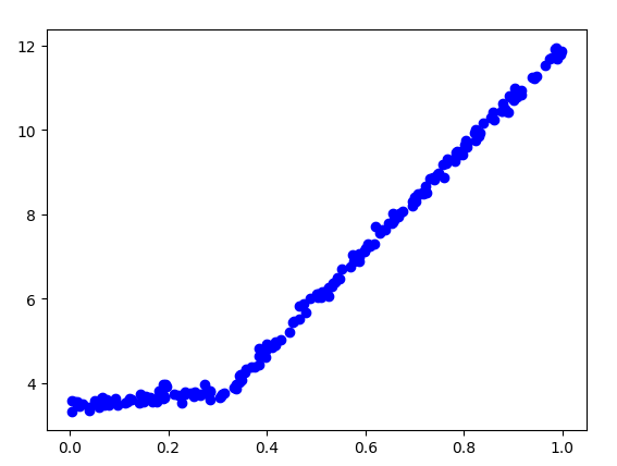
#树回归与标准回归
#用树回归进行预测
#1-回归树
def regTreeEval(model, inDat):
    return float(model)
#2-模型树
def modelTreeEval(model, inDat):
    n = shape(inDat)[1]
    X = mat(ones((1, n + 1)))
    X[:, 1:n + 1] = inDat
    return float(X * model)
#对于输入的单个数据点，treeForeCast返回一个预测值。
def treeForeCast(tree, inData, modelEval=regTreeEval):#指定树类型
    if not isTree(tree): return modelEval(tree, inData)
    if inData[tree['spInd']] > tree['spVal']:
        if isTree(tree['left']):#有左子树 递归进入子树
            return treeForeCast(tree['left'], inData, modelEval)
        else:#不存在子树 返回叶节点
            return modelEval(tree['left'], inData)
    else:
        if isTree(tree['right']):
            return treeForeCast(tree['right'], inData, modelEval)
        else:
            return modelEval(tree['right'], inData)
#对数据进行树结构建模
def createForeCast(tree, testData, modelEval=regTreeEval):
    m = len(testData)
    yHat = mat(zeros((m, 1)))
    for i in range(m):
        yHat[i, 0] = treeForeCast(tree, mat(testData[i]), modelEval)
    return yHat

测试创建回归树:

>>> from imp import reload
>>> reload(regTrees)
<module 'regTrees' from 'D:\Python\Mechine_learning\RegTree\regTrees.py'>
>>> from numpy import *
>>> trainMat=mat(regTrees.loadDataSet('bikeSpeedVsIq_train.txt'))
>>> testMat=mat(regTrees.loadDataSet('bikeSpeedVsIq_test.txt'))
>>> myTree=regTrees.createTree(trainMat,ops=(1,20))
>>> yHat=regTrees.createForeCast(myTree,testMat[:,0])
>>> corrcoef(yHat,testMat[:,1],rowvar=0)[0,1]
0.964085231822215

线性回归效果：

>>> ws,X,Y=regTrees.linearSolve(trainMat)
>>> ws
matrix([[37.58916794],
        [ 6.18978355]])
>>> for i in range(shape(testMat)[0]):
...  yHat[i] = testMat[i,0]*ws[1,0]+ws[0,0]
...
>>> corrcoef(yHat,testMat[:,1],rowvar=0)[0,1]
0.9434684235674766

4 CART回归树总结