首先要清楚,逻辑回归是一种分类算法。它是在线性回归模型的基础上,使用Sigmoid函数,将线性模型的预测结果转变为离散变量,从而用于处理分类问题。
1 逻辑回归原理
以二分类为例,说明逻辑回归的工作原理。由线性回归小结基础,不难得出线性回归的假设函数(h_{ heta }^{'}left ( x
ight )),在逻辑回归中,使用Sigmoid函数使得(h_{ heta }^{'}left ( x
ight ))的值在[0,1]区间内。
一般Sigmoid函数表示为:
绘图展示Sigmoid函数:
#Sigmoid function
from scipy.special import expit

def sigmoid(z):
    return 1/(1 +np.exp(-z))


def h(theta, X):
    return expit(np.dot(X, theta))


#check sigmoid function
myx = np.arange(-10, 10, 0.01)
plt.plot(myx, expit(myx))
plt.title('Sigmoid Function')
plt.show()
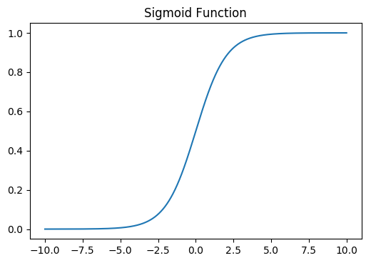
可以看到,Sigmoid函数当(z)趋于正无穷时,(gleft ( z
ight ))趋于1,当(z)趋于负无穷时,(gleft ( z
ight ))趋于0。
对于逻辑回归,令(z=h_{ heta }^{'}left ( x
ight )),则有(gleft ( z
ight )=gleft ( h_{ heta }^{'}left ( x
ight )
ight )=frac{1}{1+e^{-h_{ heta }^{'}left ( x
ight )}}),其中,$h_{ heta }^{'}left ( x
ight )=x heta $。因此,逻辑回归的模型为:
结合Sigmoid函数,理解逻辑回归模型如何实现分类问题的。此时,(h_{ heta }left ( x
ight ))为模型输出,把它当作某一分类的概率值,赋予其概率含义。当(h_{ heta }left ( x
ight )>0.5)时,(x heta >0),则(y)为1,当(h_{ heta }left ( x
ight )<0.5)时,(x heta <0),则(y)为0,如此实现了分类问题。
逻辑回归模型的矩阵形式为:
因此,(y)取1的概率等于(h_{ heta }left ( x ight )),取0的概率为(1-h_{ heta }left ( x ight )),即:
似然函数:
对数似然函数:
损失函数:
损失函数的矩阵形式为:
逻辑回归的优化目标:
2 逻辑回归算法
由于(frac{partial J( heta )}{partial heta }=X^{T}(h_{ heta }(X)-Y))
梯度下降法中$ heta $的迭代公式为:
3 逻辑回归代码实现
3.1 训练算法:使用梯度上升找到最佳参数
#Logistic 回归梯度上升优化算法
from numpy import *
def loadDataSet():
    dataMat = []; labelMat = []
    fr = open('testSet.txt')
    for line in fr.readlines():
        lineArr = line.strip().split()
        dataMat.append([1.0, float(lineArr[0]), float(lineArr[1])])
        labelMat.append(int(lineArr[2]))
    return dataMat,labelMat

def sigmoid(inX):
    return 1.0/(1+exp(-inX))

def gradAscent(dataMatIn, classLabels):
    dataMatrix = mat(dataMatIn)
    labelMat = mat(classLabels).transpose()
    m,n = shape(dataMatrix)
    alpha = 0.001
    maxCycles = 500
    weights = ones((n,1))
    for k in range(maxCycles):
        h = sigmoid(dataMatrix*weights)
        error = (labelMat - h)
        weights = weights + alpha*dataMatrix.transpose()*error
    return weights

dataArr, labelMat = loadDataSet()
print(gradAscent(dataArr, labelMat))
#输出
[[ 4.12414349]
[ 0.48007329]
[-0.6168482 ]]
4.2 分析数据:画出决策边界
#画出数据集和Logistic回归最佳拟合直线的函数
#绘制图像
import matplotlib.pyplot as plt
def plotBestFit(wei):
    weights = wei.getA()
    dataMat,labelMat=loadDataSet()
    dataArr=array(dataMat)
    n=shape(dataMat)[0]          #样本数目
    xcord1=[]; ycord1=[]
    xcord2=[]; ycord2=[]
    for i in range(n):
        if int(labelMat[i])==1:
            xcord1.append(dataArr[i,1])
            ycord1.append(dataArr[i,2])
        else:
            xcord2.append(dataArr[i,1])
            ycord2.append(dataArr[i,2])
    fig=plt.figure()
    ax=fig.add_subplot(111)
    ax.scatter(xcord1,ycord1,s=20,c='r',marker='s')
    ax.scatter(xcord2,ycord2,s=20,c='g')
    x = arange(-3.0, 3.0, 0.1)  # 直线x坐标的取值范围
    y = (-weights[0] - weights[1] * x) / weights[2]  # 直线方程
    plt.title('DataSet')
    ax.plot(x, y)
    plt.xlabel('X1');
    plt.ylabel('X2');
    plt.show()
dataArr, labelMat = loadDataSet()
weights = gradAscent(dataArr, labelMat)
plotBestFit(weights)
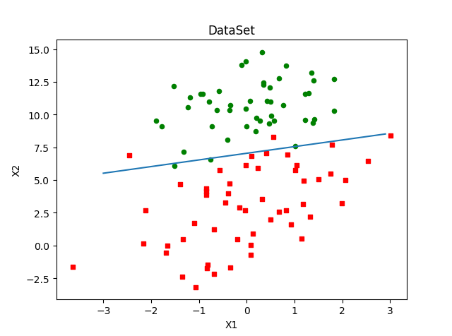
梯度上升算法在500次迭代后得到的Logistic回归最佳拟合直线:
4.3 训练算法:随机梯度上升
梯度上升算法在每次更新回归系数时都需要遍历整个数据集,该方法在处理100个左右的数据集时尚可,但如果有数十亿样本和成千上万的特征,那么该方法的计算复杂度就太高了。一种改进方法是一次仅用一个样本点来更新回归系数,该方法称为随机梯度上升算法。
#随机梯度上升算法
def stocGradAscent0(dataMatrix, classLabels):
    m,n = shape(dataMatrix)
    alpha = 0.01
    weights = ones(n)
    for i in range(m):
        h = sigmoid(sum(dataMatrix[i]*weights))
        error = classLabels[i] - h
        weights = weights + alpha*error*dataMatrix[i]
    return weights

def plotBestFit(wei):

    dataMat,labelMat=loadDataSet()
    dataArr=array(dataMat)
    n=shape(dataMat)[0]          #样本数目
    xcord1=[]; ycord1=[]
    xcord2=[]; ycord2=[]
    for i in range(n):
        if int(labelMat[i])==1:
            xcord1.append(dataArr[i,1])
            ycord1.append(dataArr[i,2])
        else:
            xcord2.append(dataArr[i,1])
            ycord2.append(dataArr[i,2])
    fig=plt.figure()
    ax=fig.add_subplot(111)
    ax.scatter(xcord1,ycord1,s=20,c='r',marker='s')
    ax.scatter(xcord2,ycord2,s=20,c='g')
    x = arange(-3.0, 3.0, 0.1)  # 直线x坐标的取值范围
    y = (-weights[0] - weights[1] * x) / weights[2]  # 直线方程
    plt.title('DataSet')
    ax.plot(x, y)
    plt.xlabel('X1');
    plt.ylabel('X2');
    plt.show()
dataMat, labelMat = loadDataSet()
weights = stocGradAscent0(array(dataMat), labelMat)
plotBestFit(weights)
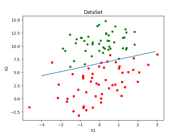
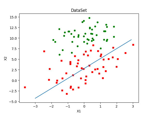
分类器错分了三分之一的样本:
直接比较随机梯度上升和梯度上升的代码结果是不公平的,后者的结果是在整个数据集上迭代了500次才得到的。一个判断优化算法优劣的可靠方法是看它是否收敛,也就是说参数是否达到了稳定值,是否还会不断地变化?对此,我们在程序清单5-3中随机梯度上升算法上做了些修改,使其在整个数据集上运行200次。最终绘制的三个回归系数的变化情况
#调整梯度上升和随机梯度上升函数
def gradAscent(dataMatIn,classlabels):
    dataMatrix=mat(dataMatIn)
    labelMat=mat(classlabels).T
    m,n=shape(dataMatrix)
    alpha=0.01
    maxCycles=500
    weights=ones((n,1))
    weights_array=array([])
    for k in range(maxCycles):
        h=sigmoid(dataMatrix*weights)
        error=labelMat-h
        weights=weights+alpha*dataMatrix.T*error
        weights_array=append(weights_array,weights)    #一行
    weights_array=weights_array.reshape(maxCycles,n)
    return weights.getA(),weights_array

def stocGradAscent1(dataMatrix,classLabels,numIter=150):
    m,n=shape(dataMatrix)
    weights=ones(n)
    weights_array=array([])
    for j in range(numIter):
        dataIndex=list(range(m))
        for i in range(m):
            alpha=4/(1.0+j+i)+0.01
            randIndex=int(random.uniform(0,len(dataIndex)))
            h=sigmoid(sum(dataMatrix[randIndex]*weights))
            error=classLabels[randIndex]-h
            weights=weights+alpha*error*dataMatrix[randIndex]
            weights_array=append(weights_array,weights,axis=0)
            del(dataIndex[randIndex])
    weights_array=weights_array.reshape(numIter*m,n)
    return weights,weights_array

#绘制回归系数与迭代次数的关系
plt.rcParams['font.sans-serif']=['SimHei']
plt.rcParams['axes.unicode_minus']=False
def plotWeights(weights_array1,weights_array2):
    #画布分成三行两列
    fig,axs=plt.subplots(nrows=3,ncols=2,sharex=False,sharey=False,figsize=(20,10))
    x1=arange(0,len(weights_array1),1)
    #绘制w0与迭代次数的关系
    axs[0][0].plot(x1,weights_array1[:,0])
    axs0_title_text=axs[0][0].set_title('梯度上升算法:回归系数与迭代次数关系')
    axs0_ylabel_text=axs[0][0].set_ylabel('W0')
    plt.setp(axs0_title_text,size=20,weight='bold',color='black')
    plt.setp(axs0_ylabel_text,size=20,weight='bold',color='black')
    #绘制w1与迭代次数关系
    axs[1][0].plot(x1,weights_array1[:,1])
    axs1_ylabel_text=axs[1][0].set_ylabel('W1')
    plt.setp(axs1_ylabel_text,size=20,weight='bold',color='black')
    #绘制w2与迭代次数关系
    axs[2][0].plot(x1,weights_array1[:,2])
    axs2_xlabel_text=axs[2][0].set_title('迭代次数')
    axs2_ylabel_text=axs[2][0].set_ylabel('W2')
    plt.setp(axs2_xlabel_text,size=20,weight='bold',color='black')
    plt.setp(axs2_ylabel_text,size=20,weight='bold',color='black')

    x2=arange(0,len(weights_array2),1)
    #绘制w0与迭代次数关系
    axs[0][1].plot(x2,weights_array2[:,0])
    axs0_title_text=axs[0][1].set_title('随机梯度上升算法:回归系数与迭代次数关系')
    axs0_ylabel_text=axs[0][1].set_ylabel('W0')
    plt.setp(axs0_title_text,size=20,weight='bold',color='black')
    plt.setp(axs0_ylabel_text,size=20,weight='bold',color='black')
    #绘制w1与迭代次数关系
    axs[1][1].plot(x2,weights_array2[:,1])
    axs1_ylabel_text=axs[1][1].set_ylabel('W1')
    plt.setp(axs1_ylabel_text,size=20,weight='bold',color='black')
    #绘制w2与迭代次数关系
    axs[2][1].plot(x2,weights_array2[:,2])
    axs2_xlabel_text=axs[2][1].set_title('迭代次数')
    axs2_ylabel_text=axs[2][1].set_ylabel('W2')
    plt.setp(axs2_xlabel_text,size=20,weight='bold',color='black')
    plt.setp(axs2_ylabel_text,size=20,weight='bold',color='black')

    plt.show()
# 绘图
dataMat, labelMat = loadDataSet()
weights1, weights_array1 = gradAscent(dataMat, labelMat)
weights2, weights_array2 = stocGradAscent1(array(dataMat), labelMat)
plotWeights(weights_array1, weights_array2)

#改进的随机梯度上升算法
import random

def stocGradAscent1(dataMatrix,classLabels,numIter=150):
    m,n=shape(dataMatrix)
    weights=ones(n)
    for j in range(numIter):
        dataIndex=list(range(m))
        for i in range(m):
            alpha=4/(1.0+j+i)+0.01            #每次调整alpha值
            randIndex=int(random.uniform(0,len(dataIndex))) #随机选取样本,可以减少周期性波动
            h=sigmoid(sum(dataMatrix[randIndex]*weights))   #梯度上升这里是向量,随机梯度上升数据类型都是数值
            error=classLabels[randIndex]-h
            weights=weights+alpha*error*dataMatrix[randIndex]
            del(dataIndex[randIndex])
    return weights
dataMat, labelMat = loadDataSet()
weights = stocGradAscent1(array(dataMat), labelMat)
plotBestFit(weights)