1、神经网络的计算通常包括前向传播(foward propagation)步骤和反向传播(backward propagation)的步骤;
2、数据预处理:
- X.shape:[nx,m]--->nx 是特征数,m为样本数
- Y.shape:[1,m]
- W.shape:[nx,1]
- b---->是实数
- X 数据标准化
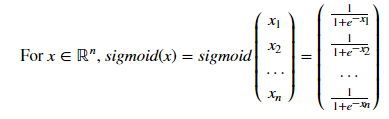
3、激励函数:
sigmoid(x)=1/(1+e-x)函数:
 1 import numpy as np
 2 def sigmoid(x):
 3     """
 4     Compute the sigmoid of x
 5
 6     Arguments:
 7     x -- A scalar or numpy array of any size
 8
 9     Return:
10     s -- sigmoid(x)
11     """
12
13
14     s = 1.0/(1+np.exp(-x))
15
16
17     return s
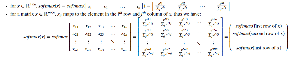
softmax函数:
 1 def softmax(x):
 2     """Calculates the softmax for each row of the input x.
 3
 4     Your code should work for a row vector and also for matrices of shape (n, m).
 5
 6     Argument:
 7     x -- A numpy matrix of shape (n,m)
 8
 9     Returns:
10     s -- A numpy matrix equal to the softmax of x, of shape (n,m)
11     """
12
13
14     # Apply exp() element-wise to x. Use np.exp(...).
15
16     x_exp = np.exp(x)
17
18     # Create a vector x_sum that sums each row of x_exp. Use np.sum(..., axis = 1, keepdims = True).
19
20     x_sum = np.sum(x_exp,axis=1,keepdims=True)
21
22     # Compute softmax(x) by dividing x_exp by x_sum. It should automatically use numpy broadcasting.
23
24     s = x_exp / x_sum
25
26
27     return s
4、二分类(Binary Classification)-Logistic Regression:
Building the parts of our algorithm:
- Define the model structure(such as number of input features)
- Initialize the model's parameters
- Loop:
- Calculate current loss(forward propagation)
- Calculate current gradient(backward propagation)
- Update parameters(gradient descent)
Forward and Backward propagation:
- You get X
- You compute A=σ(wTX+b)=(a(0),a(1),...,a(m−1),
- You calculate the cost function:J=−1/m∑mi=1y(i)log(a(i))+(1−y(i))log(1−a(i))
- Backward propagation:
-
∂J/∂w=(1/m)X(A−Y)T
-
∂J/∂b=1m∑i=1m(a(i)−y(i))
-

 1 import numpy as np
 2
 3 #define sigmoid
 4
 5 def sigmoid(z):
 6     s=1.0/(1+np.exp(z))
 7
 8 #Initializing parameters
 9
10 def initialize_with_zeros(dim):
11     w=np.zeros((dim,1))
12     b=0
13     assert(w.shape==(dim, 1))
14     assert(isinstance(b,float) or isinstance(b,int))
15     return w,b
16
17 # forward and backward propagate
18
19 def propagate(w,b,X,Y):
20         """
21     Implement the cost function and its gradient for the propagation explained above
22
23     Arguments:
24     w -- weights, a numpy array of size (num_px * num_px * 3, 1)
25     b -- bias, a scalar
26     X -- data of size (num_px * num_px * 3, number of examples)
27     Y -- true "label" vector (containing 0 if non-cat, 1 if cat) of size (1, number of examples)
28
29     Return:
30     cost -- negative log-likelihood cost for logistic regression
31     dw -- gradient of the loss with respect to w, thus same shape as w
32     db -- gradient of the loss with respect to b, thus same shape as b
33     """
34     m=X.shape[1]
35     A=sigmoid(np.dot(w.T,X))
36     cost=(-1.0/m)*np.sum(Y*np.log(A)+(1-Y)*np.log((1-A)))
37     dw=(1/m)*np.dot(X,(A-Y).T)
38     db=(1/m)*np.sum(A-Y)
39     assert(dw.shape==w.shape)
40     assert(db.type==b.type)
41     cost=np.squeeze(cost)
42     assert(cost.shape==())
43     grads={"dw":dw,
44                 "db":db}
45     return grads,cost
46
47 #using gradient descent,The goal is to learn  ww  and  bb  by minimizing the cost function  JJ . For a parameter  θθ , the update rule is  θ=θ−α dθ , where  αα  is the learning rate.
48
49 def optimize(w, b, X, Y, num_iterations, learning_rate, print_cost = False):
50     costs=[]
51     for i in range(num_iterations):
52         grads, cost = propagate(w,b,X,Y)
53         dw = grads["dw"]
54         db = grads["db"]
55         w = w - learning_rate * dw
56         b = b - learning_rate * db
57         if i%100==0:
58             costs.append(cost)
59         if print_cost and i%100==0:
60             print ("Cost after iteration %i: %f" %(i, cost))
61     params = {"w": w,
62               "b": b}
63
64     grads = {"dw": dw,
65              "db": db}
66
67     return params, grads, costs
68
69 #predict
70 def predict(w,b,X):
71     m=X.shape[1]
72     Y_prediction=np.zeros((1,m))
73     w=w.reshape(X.shape[0],1)
74     A=sigmoid(np.dot(w.T,X)+b)
75     for i in range(A.shape[1]):
76         Y_prediction[0,i]=np.where(A[0,i]>=0.5,1,0)
77     assert(Y_prediction.shape==(1,m))
78     return Y_prediction
79
80 #model
81
82 def model(X_train, Y_train, X_test, Y_test, num_iterations = 2000, learning_rate = 0.5, print_cost = False):
83      w, b = initialize_with_zeros(X_train.shape[0])
84      parameters, grads, costs = optimize(w, b, X_train, Y_train, num_iterations, learning_rate, print_cost)
85     Y_prediction_test = predict(w, b, X_test)
86     Y_prediction_train = predict(w, b, X_train)
87     print("train accuracy: {} %".format(100 - np.mean(np.abs(Y_prediction_train - Y_train)) * 100))
88     print("test accuracy: {} %".format(100 - np.mean(np.abs(Y_prediction_test - Y_test)) * 100))
89     d = {"costs": costs,
90          "Y_prediction_test": Y_prediction_test,
91          "Y_prediction_train" : Y_prediction_train,
92          "w" : w,
93          "b" : b,
94          "learning_rate" : learning_rate,
95          "num_iterations": num_iterations}
96
97     return d