Minist数据集:MNIST_data 包含四个数据文件
一、方法一:经典方法 tf.matmul(X,w)+b
import tensorflow as tf
import numpy as np
import input_data
import time

#define paramaters
learning_rate=0.01
batch_size=128
n_epochs=900

# 1.read from data file
#using TF learn built in function to load MNIST data to the folder data
mnist=input_data.read_data_sets('MNIST_data/',one_hot=True)

# 2.creat placeholders for features and label
# each img in mnist data is 28*28 ,therefor need a 1*784 tensor
# 10 classes corresponding to 0-9
X=tf.placeholder(tf.float32,[batch_size,784],name='X_placeholder')
Y=tf.placeholder(tf.float32,[batch_size,10 ],name='Y_placeholder')

# 3.creat weight and bias ,w init to random variables with mean of 0 ;
# b init to 0 ,shape of b depends on Y ,shape of w depends on the dimension of X and Y_placeholder
w=tf.Variable(tf.random_normal(shape=[784,10],stddev=0.01),name='weights')
b=tf.Variable(tf.zeros([1,10]),name="bias")

# 4.build model to predict
# the model that returns the logits ,the logits will later passed through softmax layer
logits=tf.matmul(X,w)+b

# 5.define lose function
# use cross entropy of softmax of logits as the loss function
entropy=tf.nn.softmax_cross_entropy_with_logits(logits=logits, labels=Y,name='loss')
loss=tf.reduce_mean(entropy)

# 6.define training open
# using gradient descent with learning rate of 0.01 to minimize loss
optimizer=tf.train.GradientDescentOptimizer(learning_rate).minimize(loss)

with tf.Session() as sess:
    writer=tf.summary.FileWriter('./my_graph/logistic_reg',sess.graph)

    start_time= time.time()
    sess.run(tf.global_variables_initializer())
    n_batches=int(mnist.train.num_examples/batch_size)
    for i in range(n_epochs) :  #train n_epochs times
        total_loss=0

        for _ in range(n_batches):
            X_batch,Y_batch=mnist.train.next_batch(batch_size)
            _,loss_batch=sess.run([optimizer,loss],feed_dict={X:X_batch,Y:Y_batch})
            total_loss +=loss_batch
        if i%100==0:
            print('Average loss epoch {0} : {1}'.format(i,total_loss/n_batches))

    print('Total time: {0} seconds'.format(time.time()-start_time))
    print('Optimization Finished!')

# 7.test the model
    n_batches=int(mnist.test.num_examples/batch_size)
    total_correct_preds=0
    for i in range(n_batches):
        X_batch,Y_batch=mnist.test.next_batch(batch_size)
        _,loss_batch,logits_batch=sess.run([optimizer,loss,logits],feed_dict={X:X_batch,Y:Y_batch})
        preds=tf.nn.softmax(logits_batch)
        correct_preds=tf.equal(tf.argmax(preds,1),tf.argmax(Y_batch,1))
        accuracy=tf.reduce_sum(tf.cast(correct_preds,tf.float32))
        total_correct_preds+=sess.run(accuracy)

    print('Accuracy {0}'.format(total_correct_preds/mnist.test.num_examples))

    writer.close()
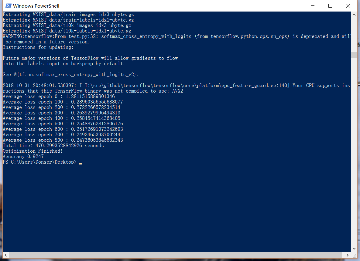
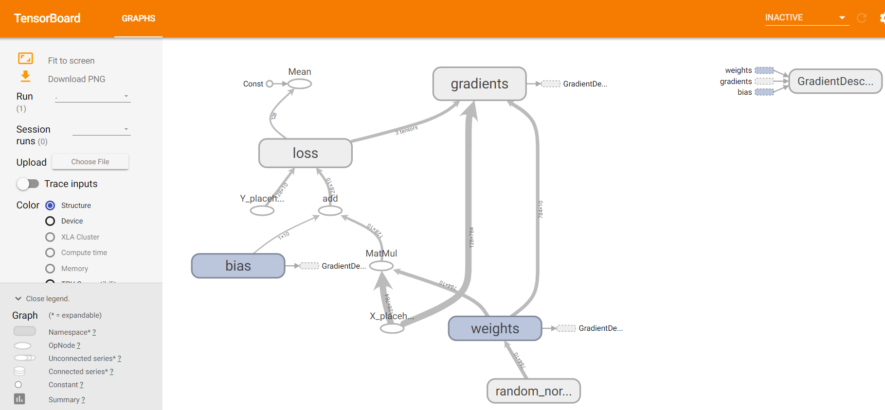
准确率大约是92%,TFboard:
二、方法二:deep learning 卷积神经网络
# load MNIST data
import input_data
mnist = input_data.read_data_sets("MNIST_data/", one_hot=True)

# start tensorflow interactiveSession
import tensorflow as tf
sess = tf.InteractiveSession()

# weight initialization
def weight_variable(shape):
    initial = tf.truncated_normal(shape, stddev=0.1)
    return tf.Variable(initial)

def bias_variable(shape):
    initial = tf.constant(0.1, shape = shape)
    return tf.Variable(initial)

# convolution
def conv2d(x, W):
    return tf.nn.conv2d(x, W, strides=[1, 1, 1, 1], padding='SAME')
# pooling
def max_pool_2x2(x):
    return tf.nn.max_pool(x, ksize=[1, 2, 2, 1], strides=[1, 2, 2, 1], padding='SAME')

# Create the model
# placeholder
x = tf.placeholder("float", [None, 784])
y_ = tf.placeholder("float", [None, 10])
# variables
W = tf.Variable(tf.zeros([784,10]))
b = tf.Variable(tf.zeros([10]))

y = tf.nn.softmax(tf.matmul(x,W) + b)
print (y)
# first convolutinal layer
w_conv1 = weight_variable([5, 5, 1, 32])
b_conv1 = bias_variable([32])
print (x)
x_image = tf.reshape(x, [-1, 28, 28, 1])
print (x_image)
h_conv1 = tf.nn.relu(conv2d(x_image, w_conv1) + b_conv1)
h_pool1 = max_pool_2x2(h_conv1)
print (h_conv1)
print (h_pool1)
# second convolutional layer
w_conv2 = weight_variable([5, 5, 32, 64])
b_conv2 = bias_variable([64])

h_conv2 = tf.nn.relu(conv2d(h_pool1, w_conv2) + b_conv2)
h_pool2 = max_pool_2x2(h_conv2)
print (h_conv2)
print (h_pool2)
# densely connected layer
w_fc1 = weight_variable([7*7*64, 1024])
b_fc1 = bias_variable([1024])

h_pool2_flat = tf.reshape(h_pool2, [-1, 7*7*64])
h_fc1 = tf.nn.relu(tf.matmul(h_pool2_flat, w_fc1) + b_fc1)
print (h_fc1)
# dropout
keep_prob = tf.placeholder("float")
h_fc1_drop = tf.nn.dropout(h_fc1, keep_prob)
print (h_fc1_drop)
# readout layer
w_fc2 = weight_variable([1024, 10])
b_fc2 = bias_variable([10])

y_conv = tf.nn.softmax(tf.matmul(h_fc1_drop, w_fc2) + b_fc2)

# train and evaluate the model
cross_entropy = -tf.reduce_sum(y_*tf.log(y_conv))
train_step = tf.train.GradientDescentOptimizer(1e-3).minimize(cross_entropy)
#train_step = tf.train.AdagradOptimizer(1e-4).minimize(cross_entropy)
correct_prediction = tf.equal(tf.argmax(y_conv, 1), tf.argmax(y_, 1))
accuracy = tf.reduce_mean(tf.cast(correct_prediction, "float"))
sess.run(tf.global_variables_initializer())
writer=tf.summary.FileWriter('./my_graph/mnist_deep',sess.graph)

# Train
tf.initialize_all_variables().run()
for i in range(1000):
    batch_xs, batch_ys = mnist.train.next_batch(100)
    #print (batch_xs.shape,batch_ys)
    if i % 100 == 0:
        train_accuracy = accuracy.eval(feed_dict={x: batch_xs, y_: batch_ys, keep_prob:0.5})
        print (("step %d, train accuracy %g" % (i, train_accuracy)))
    train_step.run({x: batch_xs, y_: batch_ys, keep_prob:0.5})
    #print(accuracy.eval({x: mnist.test.images, y_: mnist.test.labels}))

# Test trained model
print( ("python_base accuracy %g" % accuracy.eval(feed_dict={x:mnist.test.images[0:500], y_:mnist.test.labels[0:500], keep_prob:0.5})))

writer.close()
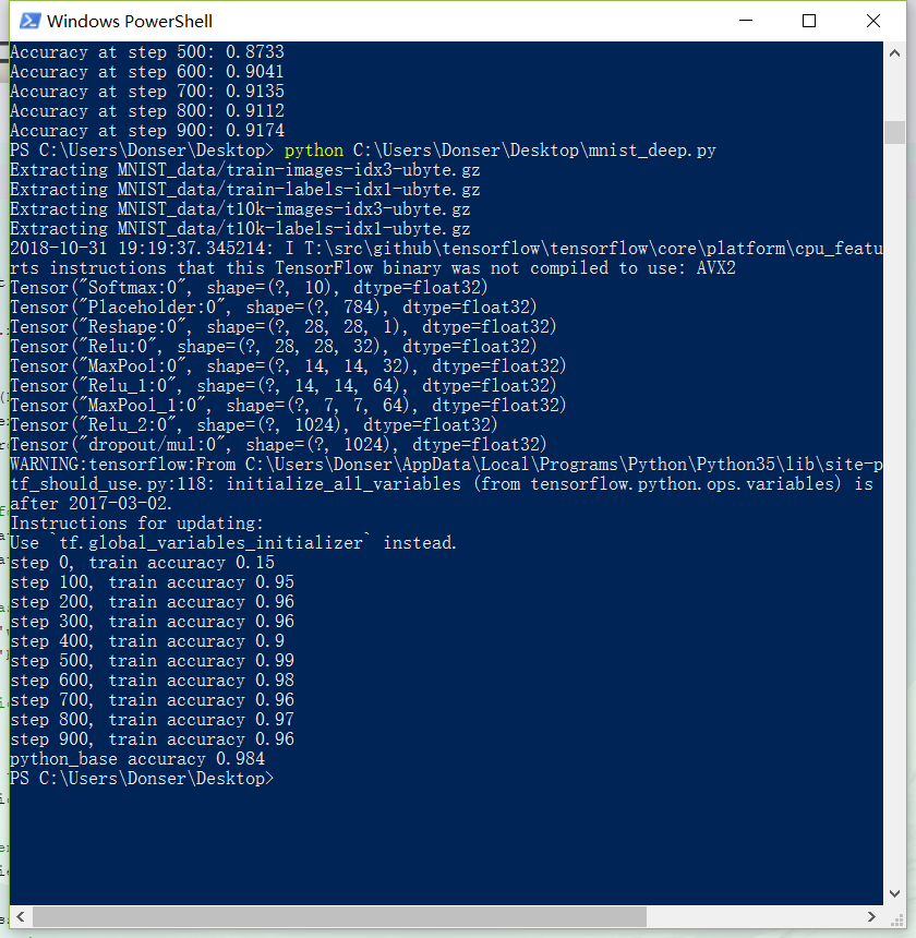
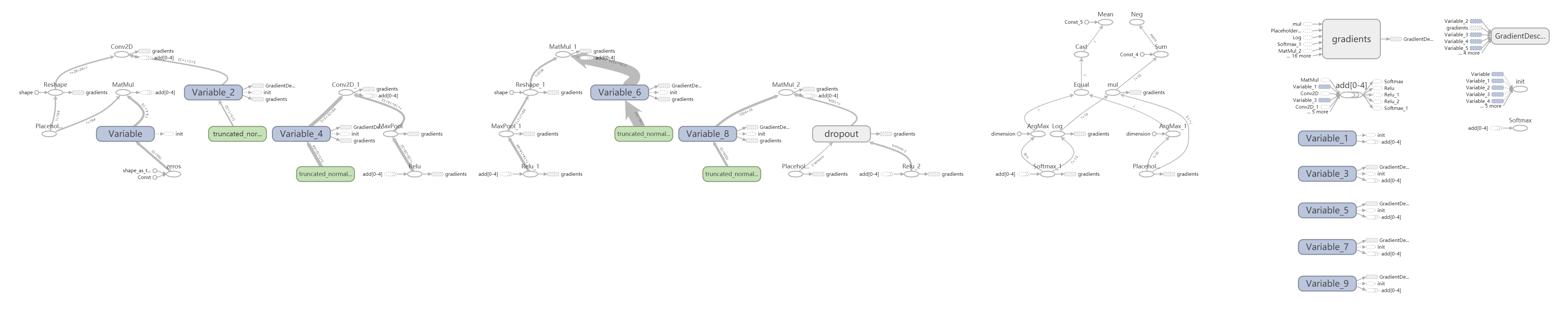
准确率达到98%,Board:
三、第三种 使用minist数据集做图像去噪
from keras.datasets import mnist
from keras.layers import Input, Dense
from keras.models import Model
from keras.layers import Input, Dense, Conv2D, MaxPooling2D, UpSampling2D
import numpy as np
from keras.callbacks import TensorBoard
import matplotlib.pyplot as plt


(x_train, _), (x_test, _) = mnist.load_data()

x_train = x_train.astype('float32') / 255.
x_test = x_test.astype('float32') / 255.
x_train = np.reshape(x_train, (len(x_train), 28, 28, 1))  # adapt this if using `channels_first` image data format
x_test = np.reshape(x_test, (len(x_test), 28, 28, 1))  # adapt this if using `channels_first` image data format

noise_factor = 0.5
x_train_noisy = x_train + noise_factor * np.random.normal(loc=0.0, scale=1.0, size=x_train.shape)
x_test_noisy = x_test + noise_factor * np.random.normal(loc=0.0, scale=1.0, size=x_test.shape)

x_train_noisy = np.clip(x_train_noisy, 0., 1.)
x_test_noisy = np.clip(x_test_noisy, 0., 1.)
x_train_noisy = x_train_noisy.astype(np.float)
x_test_noisy = x_test_noisy.astype(np.float)


input_img = Input(shape=(28, 28, 1))  # adapt this if using `channels_first` image data format

x = Conv2D(32, (3, 3), activation='relu', padding='same')(input_img)
x = MaxPooling2D((2, 2), padding='same')(x)
x = Conv2D(32, (3, 3), activation='relu', padding='same')(x)
encoded = MaxPooling2D((2, 2), padding='same')(x)

# at this point the representation is (7, 7, 32)

x = Conv2D(32, (3, 3), activation='relu', padding='same')(encoded)
x = UpSampling2D((2, 2))(x)
x = Conv2D(32, (3, 3), activation='relu', padding='same')(x)
x = UpSampling2D((2, 2))(x)
decoded = Conv2D(1, (3, 3), activation='sigmoid', padding='same')(x)

autoencoder = Model(input_img, decoded)
autoencoder.compile(optimizer='adadelta', loss='binary_crossentropy')

autoencoder.fit(x_train_noisy, x_train,
                epochs=100,
                batch_size=128,
                shuffle=True,
                validation_data=(x_test_noisy, x_test),
                callbacks=[TensorBoard(log_dir='/tmp/tb', histogram_freq=0, write_graph=True)])


n = 10
plt.figure(figsize=(20, 4))
for i in range(n):
#noisy data
    ax = plt.subplot(3, n, i+1)
    plt.imshow(x_test_noisy[i].reshape(28, 28))
    plt.gray()
    ax.get_xaxis().set_visible(False)
    ax.get_yaxis().set_visible(False)
#predict
    ax = plt.subplot(3, n, i+1+n)
    decoded_img = autoencoder.predict(x_test_noisy)
    plt.imshow(decoded_img[i].reshape(28, 28))
    plt.gray()
    ax.get_yaxis().set_visible(False)
    ax.get_xaxis().set_visible(False)
#original
    ax = plt.subplot(3, n, i+1+2*n)
    plt.imshow(x_test[i].reshape(28, 28))
    plt.gray()
    ax.get_yaxis().set_visible(False)
    ax.get_xaxis().set_visible(False)
plt.show()
使用了keras,见官网 https://blog.keras.io/building-autoencoders-in-keras.html
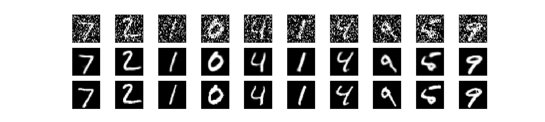
第一行是加了噪声的图,第二行是去噪以后的图,第三行是原图,回复效果较好
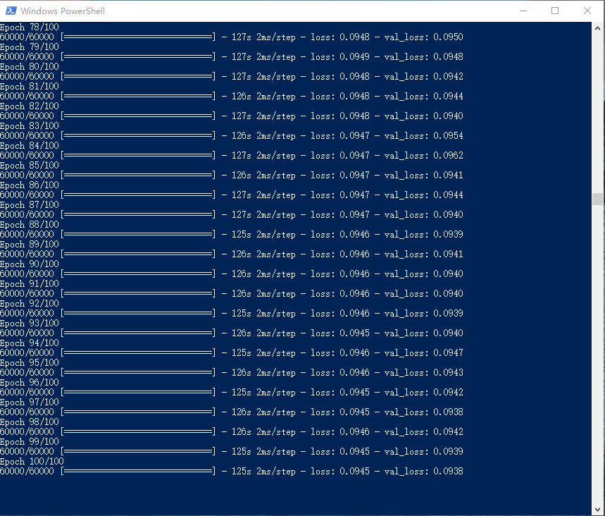
125s跑一个epoch,100组三个半小时搞定
tensorboard --logdir=/tmp/tb