机器学习的最实际应用涉及目标结果所依赖的多个功能。类似地,在回归分析问题中,有时目标结果取决于众多功能。多元线性回归是解决此类问题的一种可行解决方案。在本文中,我将讨论多元(多种功能)线性回归,从头开始的Python实现,在实际问题上的应用和性能分析。
由于它是一种“线性”回归技术,因此在假设的框架中将仅采用每个特征的线性项。令x_1,x_2,…x_n为目标结果所依赖的要素。然后,关于多元线性回归的假设:

其中theta_0,theta_1,theta_2,theta_3,…。,theta_n是参数
同样,上述假设也可以根据矢量代数重新构建:

还有一个与假设相关的成本函数(或损失函数),取决于参数theta_0,theta_1,theta_2,…,theta_n。
这里的成本函数与多项式回归[1]的情况相同。
因此,这些参数theta_0,theta_1,theta_2,...,theta_n必须采用这样的值,对于这些值,成本函数(或简称为cost)达到其可能的最小值。换句话说,必须找出成本函数的最小值。
在这种情况下,批梯度下降可以用作优化策略。
使用批量梯度下降实现多元线性回归:
通过创建3个模块来完成实施,每个模块用于在培训过程中执行不同的操作。
=> hypothesis():给定theta(theta_0,theta_1,theta_2,theta_3,…。,theta_n),矩阵中的特征,尺寸为[m X的X],它是用于计算和输出目标变量的假设值的函数(n + 1)],其中m是样本数,n是特征数。下面给出了hypothesis()的实现:
def hypothesis(theta, X, n):
    h = np.ones((X.shape[0],1))
    theta = theta.reshape(1,n+1)
    for i in range(0,X.shape[0]):
        h[i] = float(np.matmul(theta, X[i]))
    h = h.reshape(X.shape[0])
    return h
=> BGD():该函数执行批量梯度下降算法,并采用theta的当前值(theta_0,theta_1,…,theta_n),学习率(alpha),迭代次数(num_iters),假设值列表所有样本(h),特征集(X),目标变量集(y)和特征数(n)作为输入,并输出优化的theta(theta_0,theta_1,theta_2,theta_3,…,theta_n)以及成本历史记录或包含所有迭代中成本函数值的成本。BGD()的实现如下:
def BGD(theta, alpha, num_iters, h, X, y, n):
    cost = np.ones(num_iters)
    for i in range(0,num_iters):
        theta[0] = theta[0] - (alpha/X.shape[0]) * sum(h - y)
        for j in range(1,n+1):
            theta[j] = theta[j] - (alpha/X.shape[0]) * sum((h-y) * X.transpose()[j])
        h = hypothesis(theta, X, n)
        cost[i] = (1/X.shape[0]) * 0.5 * sum(np.square(h - y))
    theta = theta.reshape(1,n+1)
    return theta, cost
=> linear_regression():它是主要函数,将特征矩阵(X),目标变量矢量(y),学习率(alpha)和迭代次数(num_iters)作为输入,并输出最终的优化theta,即成本函数在批次梯度下降之后几乎达到最小值的[ theta_0,theta_1,theta_2,theta_3,….theta_n ] 值,以及cost,它存储每次迭代的成本值。
def linear_regression(X, y, alpha, num_iters):
    n = X.shape[1]
    one_column = np.ones((X.shape[0],1))
    X = np.concatenate((one_column, X), axis = 1)
    # initializing the parameter vector...
    theta = np.zeros(n+1)
    # hypothesis calculation....
    h = hypothesis(theta, X, n)
    # returning the optimized parameters by Gradient Descent...
    theta, cost = BGD(theta,alpha,num_iters,h,X,y,n)
    return theta, cost
问题陈述:“ 给定房屋的大小和卧室的数量,分析并预测房屋的可能价格”
数据读入Numpy数组:
data = np.loadtxt('data1.txt', delimiter=',')
X_train = data[:,[,1]]
y_train = data[:,2]
特征归一化或特征缩放:
这涉及缩放特征以进行快速有效的计算。

标准功能缩放策略 (主要用来处理量纲)
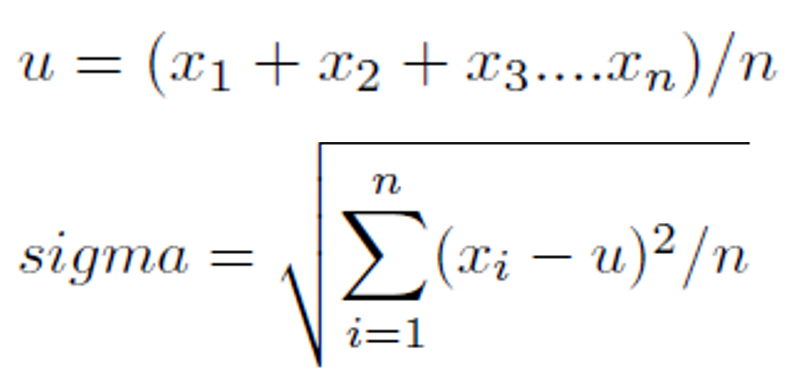
其中u是均值,sigma是标准差:
功能缩放的实现:
mean = np.ones(X_train.shape[1])
std = np.ones(X_train.shape[1])
for i in range(0, X_train.shape[1]):
    mean[i] = np.mean(X_train.transpose()[i])
    std[i] = np.std(X_train.transpose()[i])
    for j in range(0,X_train.shape[0]):
        X_train[j][i] = (X_train[j][i] - mean[i])/std[i]
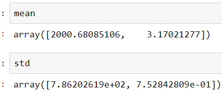
这里,
- “房屋大小(以平方英尺为单位)”或F1:2000.6808
- “卧房数”或F2的平均值:3.1702
- F1的标准偏差:7.86202619e + 02
- F2的标准偏差:7.52842809e-01
#调用与主要功能learning_rate = 0.0001和
#num_iters = 300000
theta, cost = linear_regression(X_train, y_train, 0.0001, 30000)
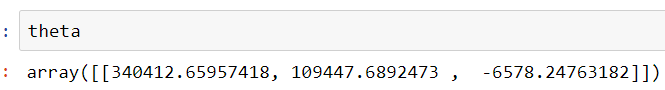
多元线性回归后的theta
在逐批迭代的批次梯度下降过程中降低了成本。借助“线曲线”可以显示成本的降低。
将matplotlib.pyplot导入为plt
cost = list(cost)
n_iterations = [x for x in range(1,30001)]
plt.plot(n_iterations, cost)
plt.xlabel('No. of iterations')
plt.ylabel('Cost')
