第3章 探索数据
本章会介绍一些技术,帮助你对一个银行营销电话的数据进行分类。你将学习以下主题:
·测试并比较模型
·朴素贝叶斯分类器
·将逻辑回归作为通用分类器使用
·将支持向量机用作分类引擎
·使用决策树进行分类
·使用随机森林预测订阅者
·使用神经网络对呼叫进行分类
3.1导论
本章中,我们会对一个银行的营销电话进行分类,看看一个呼叫会不会带来一个信用卡业务。本文引用《A Data-Driven Approach to Predict the Success of Bank Telemarketing》中的数据,这本书可在http://archive.ics.uci.edu/ml/datasets/Bank+Marketing上找到。
为了能在我们的模型中使用,我们转换了数据。数据字典在/Data/Chapter03/bank_contacts_data_dict.txt。
3.2测试并比较模型
独立安装 pandas
>pip install pandas
独立安装 scikit-learn
>pip install scikit-learn
pandas让计算你所用模型的性能指标变得极其容易。我们使用下面的代码衡量模型的能力(Codes文件夹根目录下的helper.py文件):
 1 import sklearn.metrics as mt
 2
 3 def printModelSummary(actual, predicted):
 4     '''
 5         Method to print out model summaries
 6     '''
 7     print('Overall accuracy of the model is {0:.2f} percent'
 8         .format(
 9             (actual == predicted).sum() /
10             len(actual) * 100))
11     print('Classification report:
',
12         mt.classification_report(actual, predicted))
13     print('Confusion matrix:
',
14         mt.confusion_matrix(actual, predicted))
15     print('ROC: ', mt.roc_auc_score(actual, predicted))
16
原理
首先,我们从scikit-learn导入了metrics模块。然后,我们输出模型总体上的精确度。这是统计我们的模型与实际分类一致的次数((actual==predicted).sum()),再除以测试样本的规模(len(actual)*100)得到的。这告诉了我们总体上成功的比例。如果独立变量的分布不对称,那么这个维度不能用来评估你的模型。
.confusion_matrix方法以一种很清晰的方式衡量我们的模型——矩阵的每一行代表着模型弄错(或预测对)的次数:
/*
Consusion matrix:
{[10154 1816]
[559,946]}
*/
第一行,很明显一共是10154+1816=11970的实际观测值,其属于0这一类。其中,10154是正确预测的数目(我们把这种情况称作true negative,因为这代表着电话并没有带来信用卡业务),1816是错误预测的数目(我们把这种情况称作false positive,这类电话被我们的模型当成了“带来了信用卡业务”,实际上并没有)。
第二行展示了模型成功预测产出的次数:559次错误(称作false negative,电话带来了信用卡业务,而模型认为没有),946次正确(称作true positive,电话带来了信用卡业务,与模型的结论一致)。
这些数值可用于计算一些指标。使用.classification_report(...)方法生成这些指标:

精确率(Precision)衡量的是,当样本不是正类时,模型不将样本预测为正类的能力。这是true positive(946)与所有预测为正类的数量(1816+946)的比值:这里是0.34,相当低。也可以为负类计算相对应的值:10154/(10154+559)=0.95。总体的精确率是个体精确率的加权平均,权重就是支持度。支持度(Support)是样本中各分类的实际数目。
召回率(Recall)可被看作模型找出所有正类的能力。这是真阳性对真阳性与假阴性之和的比值:946/(946+559)=0.63。同样地,可以用真阴性比上真阴性和假阳性之和,得到类别0的召回率。总体的召回率是各类别召回率的加权平均,权重是支持度。
综合评价指标(F1-score)是精确率和召回率的调和平均。即精确率和召回率乘积的两倍比上它们的和。用这一个指标来衡量模型表现的好坏。
用于评估模型表现的最后一个指标是ROC曲线(Receiver Operating Characteristic)。ROC曲线将模型的表现可视化(对分类的比例不敏感)。换句话说,这条曲线相当于以更多假阳性的代价换取更多真阳性的权衡。我们对ROC曲线下方的面积更感兴趣。一般认为0.9到1的模型是优秀的,而0.5和0.6这种的则没什么价值——这种模型和抛硬币做决定没什么差别。
在helper.py文件中,我们放了一些后续章节常用的辅助过程。使用最多的应该就是timeit(...)装饰器了。这个装饰器可用来测量程序的运行时间:
def timeit(method):
    '''
    A decorator to time how long it takes to estimate the models
        一个用于估算模块所需时间的装饰器
    '''

    def timed(*args, **kw):
        start = time.time()
        result = method(*args, **kw)
        end = time.time()

        print('The method {0} took {1:2.2f} sec to run.'
              .format(method.__name__, end-start))
        return result

    return timed
这个装饰器返回的是timed(...)方法,这个方法测量的是一个方法执行过程的结束与开始的时间戳之差。要使用一个装饰器,我们将@timeit(或者@hlp.timeit)放在要测量的函数前面。timeit(...)方法唯一的参数,就是传递给timed(...)这个内部方法的method。timed(...)方法启动计时器,执行传递进来的函数,再打印出用了多久。
Python中的函数,也是可以传递的对象,和其他对象(比如int)没什么差别。所以,我们可以将方法作为参数传给另一个函数,并在内部使用。
关于(Python 3.7的)装饰器,可参考http://thecodeship.com/patterns/guide-to-python-function-decorators/。
参考
强烈推荐Scikit文档中关于分类器各种指标的部分:
http://scikit-learn.org/stable/modules/model_evaluation.html。
3.3朴素贝叶斯分类器
独立安装 pandas
>pip install pandas
独立安装 scikit-learn
>pip install scikit-learn
朴素贝叶斯分类器是最简单的分类技术之一。其理论基础是贝叶斯定理,在一个事件发生的情况下,求另一事件发生的概率:
P(A|B)=P(B|A)P(A)/P(B)
也就是说,我们有电话及通话方的各种特征(B),要计算电话带来信用卡业务的概率(A)。这就等价于计算:观测到的申请信用卡的频率P(A),乘以过去同意办理信用卡的通话方与电话具有这些特征的频率P(B|A),比上数据集中这些通话方与电话的频率P(B)。
本节示例需要装好pandas和scikit-learn。我们还要使用helper.py文件,所以你需要NumPy和time模块。
helper.py文件放在上一级目录,我们需要将上一层目录加到Python的环境变量中,Python会到这些路径下寻找代码:
# this is needed to load helper from the parent folder
import sys
sys.path.append('..')

# the rest of the imports
import helper as hlp
import pandas as pd
import sklearn.naive_bayes as nb
使用pandas构造朴素贝叶斯分类器只花两行代码。但到那一步之前得做点长一些的准备(classification_naiveBayes.py文件):
 1 # the file name of the dataset
 2 r_filename = '../../Data/Chapter03/bank_contacts.csv'
 3
 4
 5 # the file name of the dataset
 6 r_filename = '../../Data/Chapter03/bank_contacts.csv'
 7
 8 # read the data
 9 csv_read = pd.read_csv(r_filename)
10
11 # split the data into training(训练集) and testing(测试集)
12 train_x, train_y,
13 test_x,  test_y,
14 labels = hlp.split_data(
15     csv_read, y = 'credit_application')
16
17 # train the model 训练模型
18 classifier = fitNaiveBayes((train_x, train_y))
19
20 # classify the unseen data
21 predicted = classifier.predict(test_x)
22
23 # print out the results
24 hlp.printModelSummary(test_y, predicted)
25
26 @hlp.timeit
27 def fitNaiveBayes(data):
28     '''
29     Build the Naive Bayes classifier
30         构造朴素贝叶斯分类器
31     '''
32     # create the classifier object 构造一个分类 器对象
33     naiveBayes_classifier = nb.GaussianNB()
34
35     # fit the model 拟合模型
36     return naiveBayes_classifier.fit(data[0], data[1])
说明:
我们先从CSV文件读取数据,这一步大家应该很熟悉了(参见本书1.2节)。接着将数据拆成训练集和测试集,维持自变量(x)和因变量(y)的分离(参见本书2.8节)。
helper.py脚本的.split_data(...)方法将数据集拆成两个子集:默认情况下,2/3的数据用于训练,1/3的数据用于测试。这个方法是前一章方法略微复杂些的变体。有两个必需的参数(按顺序)是:data和y(因变量)。data参数应是pandas的DataFrame类型,y应传这个DataFrame中某列的名字。你可以用x参数传入一个列名的列表,作为指定的自变量(默认是选取除y外的所有列)(本章后面会详细讲这块)。你也可以给test_size参数传入一个0到1之间的数,以指定测试数据占的比例。
拆分完数据集,我们就可以构造分类器了。当前技巧和下一个技巧中,我们将用@hlp.timeit装饰器给不同的模型计时。
我们使用Scikit的.GaussianNB()方法构建朴素贝叶斯分类器。这个方法不用传参数。使用.fit(...)方法拟合模型;要传的第一个参数是自变量的集合,第二个参数是因变量的向量。一旦拟合,我们就向主程序返回分类器。模型就构建成功。
下面我们要测试模型。.predict(...)方法处理test_x数据集,将样本分为两个桶:一个是带来信用卡申请的电话,一个是没带来申请的电话。
Scikit中不同模型遵循同样的命名模式;这样用起来就很方便。后续用到的其他模型都有.fit(...)和.predict(...)方法,这样不用修改代码,也能很方便地测试不同的模型。
我们用之前介绍的printModelSummary(...)方法测试模型的表现(参考本书3.2节)。fitNaiveBayes(...)在平均情况下,(在我的机器上)花费0.03秒。
在你的机器上,程序运行的时间很可能不同。我们只将这个时间用作与后续介绍的方法进行比较的基准(你也该如此)。

朴素贝叶斯在很多机器学习的应用中都有运用。比如,如何分类文本:http://sebastianraschka.com/Articles/2014_naive_bayes_1.html。
3.4将逻辑回归作为通用分类器使用
独立安装 pandas
独立安装 StatsModels
>pip install StatsModels
/*
Looking in indexes: https://pypi.tuna.tsinghua.edu.cn/simple
Installing collected packages: patsy, StatsModels
Successfully installed StatsModels-0.10.2 patsy-0.5.1
FINISHED
 */
逻辑回归可能是第二广泛的回归模型(排在线性回归之后)。不过它也可用于解决分类问题。
要实践本技巧,你需要装好pandas和StatsModels。如果你使用的是Anaconda发行版Python,那么这两个模块都已预装。我们引入StatsModels的两个部分:
import statsmodels.api as sm
import statsmodels.genmod.families.links as fm
前一个允许我们选取模型,后一个允许我们指定链接函数。
类似前一招的模式,我们先导入需要的模块,读入数据,拆分数据集。然后调用fitLogisticRegression(...)方法来预测模型(classification_logistic.py文件):
@hlp.timeit
def fitLogisticRegression(data):
    '''
        Build the logistic regression classifier
        构建逻辑回归分类器
    '''
    # create the classifier object 创建分类器对象
    logistic_classifier = sm.GLM(data[1], data[0],
        family=sm.families.Binomial(link=fm.logit))

    # fit the data拟合数据
    return logistic_classifier.fit()
StatsModels模块提供了.GLM(...)方法。GLM代表广义线性模型(Generalized Linear Model)。广义线性模型是一族模型,可为其他分布生成一个线性回归(误差项的正态性假设之下)。模型可以表述为:
这里g是一个链接函数,Xβ是线性等式的集合,E(Y)是因变量的期望(把它看成一个非正态分布的平均值)。GLM用链接函数将模型与响应变量的分布关联起来。
这里有所有链接函数的列表:http://statsmodels.sourceforge.net/devel/glm.html#links。
StatsModels的.GLM(...)方法允许我们指定很多分布。在我们的例子中,应用了二项分布变量,这种变量只有两种取值:1代表带来信用卡申请的电话,0代表没带来信用卡申请的电话。这样我们就可以应用.families.Binomial(...)方法。实际上,二项分布族默认的链接函数就是logit,所以我们其实不用显式指定;我们这样做,只是为了在你要用其他链接函数时,知道怎么做。
StatsModels中实现的所有模型族列表:http://statsmodels.sourceforge.net/devel/glm.html#families。
我们更熟悉的也许是sigmoid函数,logit函数是其反函数(参见下图):
如你所见,逻辑回归的输出只能在0和1之间变化,我们可以将其作为电话转化为信用卡申请的概率;一旦高于50%,我们就认为更有可能带来信用卡申请,将其归为1,否则就归为0。下面的代码可以获得这个效果:
# classify the unseen data 对隐藏的数据分类
predicted = classifier.predict(test_x)

# assign the class指定类别
predicted = [1 if elem > 0.5 else 0 for elem in predicted]

# print out the results打印结果
hlp.printModelSummary(test_y, predicted)
我们使用列表表达式将最终的分类赋给测试数据集。然后,我们用.printModel Summary(...)方法列出模型的性能表现。逻辑回归分类器的表现要比朴素贝叶斯的好,但这是建立在更高的计算代价之上的。
与朴素贝叶斯分类器相比,我们付出了高估false positive的代价,得到的是更好的归类true positive的能力。
StatsModels的GLM分类器允许我们打印出关于回归的更详细的结果,以及系数值和它们的统计表现。在分类器上调用的.summary()方法会打印类似下图(缩略版)的结果:


   Generalized Linear Model Regression Results
==============================================================================
Dep. Variable:     credit_application   No. Observations:                27753
Model:                            GLM   Df Residuals:                    27701
Model Family:                Binomial   Df Model:                           51
Link Function:                  logit   Scale:                          1.0000
Method:                          IRLS   Log-Likelihood:                    nan
Date:                Sun, 15 Mar 2020   Deviance:                          nan
Time:                        16:56:57   Pearson chi2:                 1.90e+19
No. Iterations:                   100
Covariance Type:            nonrobust
================================================================================================
                                   coef    std err          z      P>|z|      [0.025      0.975]
------------------------------------------------------------------------------------------------
n_age                        -1.937e+13   4.09e+06  -4.74e+06      0.000   -1.94e+13   -1.94e+13
n_duration                    1.091e+16   7.63e+06   1.43e+09      0.000    1.09e+16    1.09e+16
n_pdays                      -8.708e+14   7.45e+06  -1.17e+08      0.000   -8.71e+14   -8.71e+14
n_previous                   -6.625e+12   1.39e+07  -4.76e+05      0.000   -6.63e+12   -6.63e+12
n_emp_var_rate               -3.034e+15   1.91e+07  -1.59e+08      0.000   -3.03e+15   -3.03e+15
n_cons_price_idx              7.766e+15    1.7e+07   4.57e+08      0.000    7.77e+15    7.77e+15
n_cons_conf_idx               2.743e+15   5.39e+06   5.09e+08      0.000    2.74e+15    2.74e+15
n_euribor3m                  -7.989e+15   1.43e+07  -5.57e+08      0.000   -7.99e+15   -7.99e+15
n_nr_employed                 9.976e+15   2.09e+07   4.76e+08      0.000    9.98e+15    9.98e+15
job_admin                    -3.148e+14   1.23e+06  -2.56e+08      0.000   -3.15e+14   -3.15e+14
job_blue_collar              -3.598e+14   1.34e+06  -2.68e+08      0.000    -3.6e+14    -3.6e+14
job_entrepreneur             -3.638e+14   2.19e+06  -1.66e+08      0.000   -3.64e+14   -3.64e+14
job_housemaid                -3.058e+14    2.5e+06  -1.22e+08      0.000   -3.06e+14   -3.06e+14
job_management               -3.439e+14   1.74e+06  -1.98e+08      0.000   -3.44e+14   -3.44e+14
job_retired                  -2.012e+14   2.29e+06  -8.78e+07      0.000   -2.01e+14   -2.01e+14
job_self_employed            -3.907e+14    2.2e+06  -1.78e+08      0.000   -3.91e+14   -3.91e+14
job_services                 -4.108e+14   1.58e+06   -2.6e+08      0.000   -4.11e+14   -4.11e+14
job_student                  -2.723e+14   2.86e+06  -9.53e+07      0.000   -2.72e+14   -2.72e+14
job_technician               -2.846e+14   1.41e+06  -2.01e+08      0.000   -2.85e+14   -2.85e+14
job_unemployed               -2.482e+14   2.47e+06  -1.01e+08      0.000   -2.48e+14   -2.48e+14
job_unknown                  -4.352e+14   4.24e+06  -1.03e+08      0.000   -4.35e+14   -4.35e+14
marital_divorced             -9.426e+14   2.92e+06  -3.23e+08      0.000   -9.43e+14   -9.43e+14
marital_married              -9.485e+14   2.78e+06  -3.42e+08      0.000   -9.48e+14   -9.48e+14
marital_single                -9.31e+14   2.81e+06  -3.32e+08      0.000   -9.31e+14   -9.31e+14
marital_unknown              -1.109e+15   7.48e+06  -1.48e+08      0.000   -1.11e+15   -1.11e+15
edu_basic_4y                 -3.349e+14   2.62e+06  -1.28e+08      0.000   -3.35e+14   -3.35e+14
edu_basic_6y                 -2.782e+14   2.78e+06     -1e+08      0.000   -2.78e+14   -2.78e+14
edu_basic_9y                 -3.374e+14   2.52e+06  -1.34e+08      0.000   -3.37e+14   -3.37e+14
edu_high_school              -2.794e+14   2.47e+06  -1.13e+08      0.000   -2.79e+14   -2.79e+14
edu_illiterate               -1.898e+15   1.59e+07  -1.19e+08      0.000    -1.9e+15    -1.9e+15
edu_professional_course      -3.051e+14   2.59e+06  -1.18e+08      0.000   -3.05e+14   -3.05e+14
edu_university_degree        -2.503e+14   2.46e+06  -1.02e+08      0.000    -2.5e+14    -2.5e+14
edu_unknown                  -2.477e+14   2.92e+06  -8.47e+07      0.000   -2.48e+14   -2.48e+14
default_unknown              -1.301e+14   1.07e+06  -1.22e+08      0.000    -1.3e+14    -1.3e+14
default_yes                  -9.129e+14   4.75e+07  -1.92e+07      0.000   -9.13e+14   -9.13e+14
housing_unknown               1.694e+13   1.34e+06   1.26e+07      0.000    1.69e+13    1.69e+13
housing_yes                  -3.679e+13   8.24e+05  -4.47e+07      0.000   -3.68e+13   -3.68e+13
loan_unknown                  1.694e+13   1.34e+06   1.26e+07      0.000    1.69e+13    1.69e+13
loan_yes                     -1.265e+13   1.13e+06  -1.12e+07      0.000   -1.27e+13   -1.27e+13
contact_cellular              -1.92e+15   3.79e+06  -5.07e+08      0.000   -1.92e+15   -1.92e+15
contact_telephone            -2.011e+15    4.2e+06  -4.79e+08      0.000   -2.01e+15   -2.01e+15
prev_ctc_outcome_failure     -9.593e+14   4.53e+06  -2.12e+08      0.000   -9.59e+14   -9.59e+14
prev_ctc_outcome_nonexistent -7.454e+14   4.15e+06  -1.79e+08      0.000   -7.45e+14   -7.45e+14
prev_ctc_outcome_success     -2.226e+15   4.54e+06   -4.9e+08      0.000   -2.23e+15   -2.23e+15
month_apr                    -9.509e+13   2.48e+06  -3.83e+07      0.000   -9.51e+13   -9.51e+13
month_aug                     3.182e+14   2.51e+06   1.27e+08      0.000    3.18e+14    3.18e+14
month_dec                    -1.189e+15   5.67e+06   -2.1e+08      0.000   -1.19e+15   -1.19e+15
month_jul                    -4.792e+14   2.27e+06  -2.12e+08      0.000   -4.79e+14   -4.79e+14
month_jun                    -2.196e+15   4.82e+06  -4.56e+08      0.000    -2.2e+15    -2.2e+15
month_mar                    -9.509e+14   3.41e+06  -2.79e+08      0.000   -9.51e+14   -9.51e+14
month_may                    -4.898e+14    1.5e+06  -3.26e+08      0.000    -4.9e+14    -4.9e+14
month_nov                     4.175e+14   1.96e+06   2.13e+08      0.000    4.17e+14    4.17e+14
month_oct                     2.752e+14   3.11e+06   8.84e+07      0.000    2.75e+14    2.75e+14
month_sep                     4.585e+14    3.8e+06   1.21e+08      0.000    4.58e+14    4.58e+14
dow_fri                      -8.033e+14    1.8e+06  -4.45e+08      0.000   -8.03e+14   -8.03e+14
dow_mon                      -8.761e+14   1.74e+06  -5.02e+08      0.000   -8.76e+14   -8.76e+14
dow_thu                       -7.73e+14   1.78e+06  -4.34e+08      0.000   -7.73e+14   -7.73e+14
dow_tue                      -7.526e+14   1.74e+06  -4.33e+08      0.000   -7.53e+14   -7.53e+14
dow_wed                       -7.26e+14   1.75e+06  -4.14e+08      0.000   -7.26e+14   -7.26e+14
================================================================================================
显而易见,n_age变量是不显著的,从模型中舍弃也不会丢失多少精度,而n_duration变量,既显著,又对消费者是否申请信用卡有重大影响。这样的信息有助于确定你的模型,并在移除无关(且可能引入误差的)变量后让模型更好。
你也可以使用Scikit的方法来估计一个逻辑回归分类器(classification_logistic_alternative.py文件):
/*
The method fitLogisticRegression took 0.69 sec to run.
Overall accuracy of the model is 91.15 percent
Classification report:
               precision    recall  f1-score   support

         0.0       0.93      0.98      0.95     12030
         1.0       0.68      0.40      0.50      1522

    accuracy                           0.91     13552
   macro avg       0.80      0.69      0.73     13552
weighted avg       0.90      0.91      0.90     13552

Confusion matrix:
 [[11743   287]
 [  913   609]]
ROC:  0.6881371909691387
{'n_age': 0.21385522376961028, 'n_duration': 19.191139443277162, 'n_pdays': -0.8673162838021525, 'n_previous': -0.18411649033655933, 'n_emp_var_rate': -4.665790648993948, 'n_cons_price_idx': 2.6226190540263103, 'n_cons_conf_idx': 0.1321457450143668, 'n_euribor3m': 1.2577893320833486, 'n_nr_employed': -1.0950955374646227, 'job_admin': 0.015606031742936122, 'job_blue_collar': -0.22590019775314962, 'job_entrepreneur': -0.07105552322436609, 'job_housemaid': -0.166748843709672, 'job_management': 0.0016511122208341445, 'job_retired': 0.31613911985033627, 'job_self_employed': -0.10302101859015086, 'job_services': -0.14037817943629885, 'job_student': 0.17802965024700726, 'job_technician': -0.017165213063450657, 'job_unemployed': 0.018250921784332092, 'job_unknown': 0.004532611196154809, 'marital_divorced': -0.0283747974255571, 'marital_married': 0.0557151595182598, 'marital_single': 0.13716177614661754, 'marital_unknown': -0.3545616669747635, 'edu_basic_4y': -0.23092212023892777, 'edu_basic_6y': -0.156627551097012, 'edu_basic_9y': -0.22916859893223016, 'edu_high_school': -0.17797495084025308, 'edu_illiterate': 0.7469642970378965, 'edu_professional_course': -0.06316024234627139, 'edu_university_degree': -0.03984420682156178, 'edu_unknown': -0.039326155497083, 'default_unknown': -0.30134284129316585, 'default_yes': 0.0, 'housing_unknown': -0.11542935562620459, 'housing_yes': -0.027745897790976075, 'loan_unknown': -0.11542935562620459, 'loan_yes': 0.03692190860121382, 'contact_cellular': 0.15231778645440006, 'contact_telephone': -0.3423773151898108, 'prev_ctc_outcome_failure': -0.5210489740812024, 'prev_ctc_outcome_nonexistent': -0.12607757606633352, 'prev_ctc_outcome_success': 0.4570670214120743, 'month_apr': -0.1322878780570286, 'month_aug': 0.39290453068094094, 'month_dec': -0.09699979367892911, 'month_jul': -0.017157002315930734, 'month_jun': -0.22287078365578353, 'month_mar': 1.2715744551548396, 'month_may': -0.6823130145064639, 'month_nov': -0.4443492486046949, 'month_oct': -0.08951220175145218, 'month_sep': -0.1690485920009346, 'dow_fri': -0.06432307409320341, 'dow_mon': -0.22305048792318713, 'dow_thu': 0.0069370229422389225, 'dow_tue': -0.004280105768027797, 'dow_wed': 0.09465711610671972}
*/
尽管这个方法比StatsModels的要快,但这是付出了代价的,它不能评估哪些系数是统计显著的,或哪些不是;.LogisticRegression(...)分类器不能生成这些统计数据。
这个模型的结果和StatsModels中的类似,比起朴素贝叶斯分类器,都是用召回率换精确率。
下一章节我们会介绍mlpy,一个机器学习模块。其也能用于预计线性模型:http://mlpy.sourceforge.net/docs/3.5/liblinear.html。
3.5将支持向量机用作分类引擎
支持向量机(Support Vector Machines,SVM)是一族可用于分类和回归问题的强大模型。与前面的模型不同,其通过所谓的核技巧,将输入向量隐式地映射到高维的特征空间,可以处理高度非线性的问题。更宽泛的SVM的解释参见:http://www.statsoft.com/Textbook/Support-Vector-Machines。
要执行后续的技巧,你需要mlpy(Machine Learning PYthon)。mlpy不在Anaconda中,所以我们需要手动安装它。mlpy要求预装GSL(GNU Scientific Library);有些系统可能已经装了GSL,所以我推荐先装mlpy。访问http://sourceforge.net/projects/mlpy/files/,下载最新资源(mlpy-<version>.tar.gz)。
注意这个地址只有32位,且只支持python3.3。
试着用pip直接安装:
pip install mlpy
/*
Looking in indexes: https://pypi.tuna.tsinghua.edu.cn/simple
Collecting mlpy
.........
ERROR: Command errored out with exit status 1: 'd:	oolspython37python.exe' -u -c 'import sys, setuptools, tokenize; sys.argv[0] = '"'"'d:\Temp\pip-install-hkwwru7x\mlpy\setup.py'"'"'; __file__='"'"'d:\Temp\pip-install-hkwwru7x\mlpy\setup.py'"'"';f=getattr(tokenize, '"'"'open'"'"', open)(__file__);code=f.read().replace('"'"'
'"'"', '"'"'
'"'"');f.close();exec(compile(code, __file__, '"'"'exec'"'"'))' install --record 'd:Temppip-record-f_wkvunvinstall-record.txt' --single-version-externally-managed --compile Check the logs for full command output.
    Running setup.py install for mlpy: finished with status 'error'
FINISHED
 */
解决方案:从非官方下载64位mlpy-3.5.0-cp37-cp37m-win_amd64.whl文件,python3.7命令行下手工安装即可。
下载地址:https://www.lfd.uci.edu/~gohlke/pythonlibs/#mlpy
注意,本章SVM代码还是运行32位能够通过。64位不行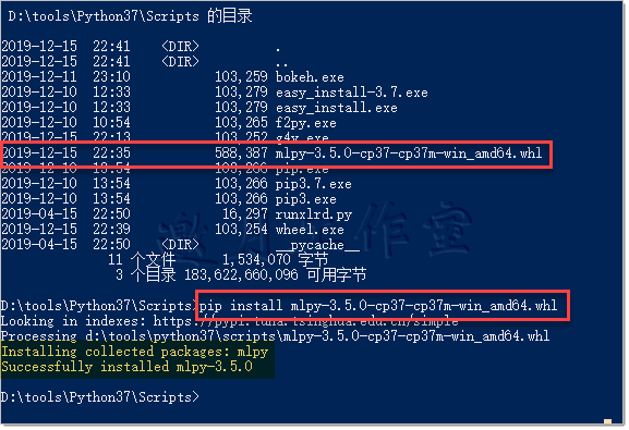
pip install gsl
/*
Looking in indexes: https://pypi.tuna.tsinghua.edu.cn/simple
Collecting gsl
  Downloading https://pypi.tuna.tsinghua.edu.cn/packages/ee/1e/14d4c4657bc7130b900c65033861ee0db508d2d9206f4223f5da7c855acc/gsl-0.0.3-py3-none-any.whl
Installing collected packages: gsl
Successfully installed gsl-0.0.3
FINISHED
 */
用mlpy构造SVM分类器很简单。你只要指定SVM的类型和它的核(classification_svm.py文件):
def fitRBFSVM(data):
    '''
    Build the linear SVM classifier
            构建线性SVM分类器
    '''
    # create the classifier object 构建分类器对象
    svm = ml.LibSvm(svm_type='c_svc',
        kernel_type='linear', C=20.0)

    # fit the data应用数据
    svm.learn(data[0],data[1])

    #return the classifier返回分类器
    return svm
原理:首先,我们加载mlpy。构建模型从调用.LibSvm(...)方法开始。我们指定的第一个参数是svm_type。c_svc指定的是C支持向量机分类器;C参数补偿了误差项。你也可以使用nu_svc参数,nu参数控制了你的样本中(最多)允许多少错误分类,以及你的观察值中(最少)有多少能成为支持向量。
顾名思义,kernel_type指定的是核的类型。我们可以选择线性、多项式、RBF(Radial Basis Functions,径向基函数)或S函数。根据你选择的核,模型会试着应用直线、多段线或者非线性的形状,来给我们的类别做最好的区分。
线性核适用于线性可分的问题,RBF可用于寻找类别之间高度非线性的界限。参考这里的展示:http://www.cs.cornell.edu/courses/cs578/2003fa/slides_sigir03_tutorial-modified.v3.pdf。
指定了模型之后,我们让它从数据中学习(.learn(...))支持向量。要使用一个RBF版本的模型,我们可以指定svm对象:
  # create the classifier object 构建分类器对象
    svm = ml.LibSvm(svm_type='c_svc', kernel_type='rbf',
        gamma=0.001, C=20.0)
这里的gamma参数指定了单个支持向量可影响的范围。你可以在这里看看gamma和C参数的关系:http://scikit-learn.org/stable/auto_examples/svm/plot_rbf_parameters.html。
目前为止,介绍的分类方法中,SVM最慢。性能也不如逻辑回归分类器。这可不是说逻辑回归就是分类问题的万能解药了。对于这个特定的数据集,逻辑回归的性能比SVM好;对于其他非线性问题,SVM也许更适合,也许会有优于逻辑回归分类器的性能。这也能从我们的SVM测试中观察到:线性核SVM的表现优于RBF核SVM:
Tips:
/*
Exception ignored in: 'libsvm.array1d_to_node'
ValueError: Buffer dtype mismatch, expected 'int_t' but got 'long long'
64位可以安装,一直编译不过去,真是见鬼了,怀疑是64位whl有问题,待求证
*/
解决方案:从非官方下载32位mlpy-3.5.0-cp37-cp37m-win32.whl文件,python官网下载32位安装文件python-3.7.5.exe
/* D:	oolsPython37_32Scripts>dir
 驱动器 D 中的卷是 Work
 卷的序列号是 9E78-6D56

 D:	oolsPython37_32Scripts 的目录

2019-12-16  10:46    <DIR>          .
2019-12-16  10:46    <DIR>          ..
2019-12-16  10:43            93,042 easy_install-3.7.exe
2019-12-16  10:43            93,042 easy_install.exe
2019-12-16  10:46            93,025 f2py.exe
2019-12-16  10:45            93,029 pip.exe
2019-12-16  10:45            93,029 pip3.7.exe
2019-12-16  10:45            93,029 pip3.exe
               6 个文件        558,196 字节
               2 个目录 183,223,492,608 可用字节

D:	oolsPython37_32Scripts>pip3.7 install mlpy-3.5.0-cp37-cp37m-win32.whl
Looking in indexes: https://pypi.tuna.tsinghua.edu.cn/simple
Processing d:	oolspython37_32scriptsmlpy-3.5.0-cp37-cp37m-win32.whl
Installing collected packages: mlpy
Successfully installed mlpy-3.5.0

D:	oolsPython37_32Scripts> */
/*
The method fitLinearSVM took 139.84 sec to run.
The method fitRBFSVM took 19.29 sec to run.
Overall accuracy of the model is 90.77 percent
Classification report:
               precision    recall  f1-score   support

         0.0       0.92      0.98      0.95     11967
         1.0       0.64      0.32      0.43      1445

    accuracy                           0.91     13412
   macro avg       0.78      0.65      0.69     13412
weighted avg       0.89      0.91      0.89     13412

Confusion matrix:
 [[11707   260]
 [  978   467]]
ROC:  0.6507284883487261
Overall accuracy of the model is 90.08 percent
Classification report:
               precision    recall  f1-score   support

         0.0       0.91      0.99      0.95     11967
         1.0       0.63      0.20      0.30      1445

    accuracy                           0.90     13412
   macro avg       0.77      0.59      0.62     13412
weighted avg       0.88      0.90      0.88     13412

Confusion matrix:
 [[11797   170]
 [ 1161   284]]
ROC:  0.5911670299783458
*/
Scikit-learn也提供了预测SVM的方法(classification_svm_alternative.py文件):
def fitSVM(data):
    '''
        Build the SVM classifier
    '''
    # create the classifier object
    svm = sv.SVC(kernel='linear', C=20.0)

    # fit the data
    return svm.fit(data[0],data[1])
这个例子中用了线性核,当然,你也可以使用RBF(实际上,.SVC(...)方法默认用的就是RBF)。得到的结果类似,但是要比mlpy快。如果需要的话,你也可以列出所有支持向量的信息;这些信息存在分类器的.support_vectors属性里:
/*
The method fitSVM took 72.45 sec to run.
Overall accuracy of the model is 90.16 percent
Classification report:
               precision    recall  f1-score   support

         0.0       0.92      0.98      0.95     11952
         1.0       0.65      0.32      0.43      1564

    accuracy                           0.90     13516
   macro avg       0.79      0.65      0.69     13516
weighted avg       0.89      0.90      0.89     13516

Confusion matrix:
 [[11690   262]
 [ 1068   496]]
ROC:  0.6476072662345889
[[0.41975309 0.16510777 1.         ... 0.         0.         0.        ]
 [0.27160494 0.41337942 1.         ... 0.         0.         0.        ]
 [0.45679012 0.17141114 1.         ... 0.         0.         0.        ]
 ...
 [0.55555556 0.06689711 1.         ... 1.         0.         0.        ]
 [0.55555556 0.04229362 0.001001   ... 1.         0.         0.        ]
 [0.69135802 0.06791379 1.         ... 0.         0.         0.        ]]
*/
3.6使用决策树进行分类
决策树广泛用于解决分类问题。顾名思义,决策树是一个树状结构,由根节点向外蔓延出分支。在每个分支(决策)节点,剩余的数据以是否满足一个具体的决策标准为依据,划分为两组。这个过程重复进行,直到不能进行进一步的划分,或者终止(叶子)节点所有的样本都从属于同一个类(这时方差最小)。
要实践本技巧,你需要装好pandas和Scikit-learn。另一种方法需要mlpy。
Scikit-learn提供了DecisionTreeClassifier(...)类,我们可以用来预测决策树分类器(classification_decisionTree.py文件):
def fitDecisionTree(data):
    '''
        Build a decision tree classifier
    '''
    # create the classifier object
    tree = sk.DecisionTreeClassifier(min_samples_split=1000)

    # fit the data
    return tree.fit(data[0],data[1])
首先,我们导入sklearn.tree模块,这个模块提供DecisionTreeClassifier(...)类供我们使用。然后我们从CSV文件读入数据,将数据集拆分成训练集和测试集。我们决定只是用所有变量的一个子集。将我们想用的变量列表作为x参数传入我们的.split\_data(...)方法:
 train_x, train_y,
test_x,  test_y,
labels = hlp.split_data(
    csv_read,
    y = 'credit_application',
    x = ['n_duration','n_nr_employed',
        'prev_ctc_outcome_success','n_euribor3m',
        'n_cons_conf_idx','n_age','month_oct',
        'n_cons_price_idx','edu_university_degree','n_pdays',
        'dow_mon','job_student','job_technician',
        'job_housemaid','edu_basic_6y']
)
注意,我们的.split_data(...)方法不仅返回训练子集和测试子集,也返回各变量的标签。
现在有了训练子集和测试子集,我们可以应用决策树了:
# train the model
classifier = fitDecisionTree((train_x, train_y))
DecisionTreeClassifier(...)类有多种操作方式。这里,我们仅仅指定每个决策节点的观测值不能少于1000个。
DecisionTreeClassifier(...)类的全部参数列表,参见http://scikit-learn.org/stable/modules/generated/sklearn.tree.DecisionTreeClassifier.html。
将模型应用(.fit(...)方法)到数据上之后,我们可以将test_x数据集中的观测值归类,打印出下面的结果:
/*
The method fitDecisionTree took 0.06 sec to run.
Overall accuracy of the model is 91.26 percent
Classification report:
               precision    recall  f1-score   support

         0.0       0.94      0.96      0.95     12202
         1.0       0.64      0.55      0.59      1585

    accuracy                           0.91     13787
   macro avg       0.79      0.75      0.77     13787
weighted avg       0.91      0.91      0.91     13787

Confusion matrix:
 [[11710   492]
 [  713   872]]
ROC:  0.7549182349482967
0. n_duration: 0.5034721037471864
1. n_nr_employed: 0.3442687149792282
2. prev_ctc_outcome_success: 0.0
3. n_euribor3m: 0.041463681111437736
4. n_cons_conf_idx: 0.03422990519127428
5. n_age: 0.01335144575508925
6. month_oct: 0.009871520358454011
7. n_cons_price_idx: 0.005585809042490998
8. edu_university_degree: 0.0031636326509486726
9. n_pdays: 0.044546262351931966
10. dow_mon: 0.0
11. job_student: 2.661076258790501e-05
12. job_technician: 0.0
13. job_housemaid: 1.5845999849280513e-05
14. edu_basic_6y: 4.468049521049593e-06 */
目前为止,这是我们用过的最好的模型,精确率和召回率都很好。朴素贝叶斯虽然有类似的ROC值,其精确率却差得多(参见朴素贝叶斯分类器)。而预测决策树分类器只比朴素贝叶斯分类器稍慢。
Scikit也提供了一个很有用的.export_graphviz(...)方法,让你可以以.dot格式保存模型;.dot格式是GraphViz的本地格式:
# and export to a .dot file
sk.export_graphviz(classifier,
    out_file='../../Data/Chapter03/decisionTree/tree.dot')
.dot文件本质上是一个文本文件,不便于阅读。不过,我们可以将其可视化。你可以使用GraphViz本身,或者,在Linux或Mac OS X上,你随时可以使用dot工具。
GraphViz是一个开源可视化工具。下载地址:http://www.graphviz.org/Download.php。
要为我们的树生成一个PDF文件,只需执行下面这行命令:
/*
dot -Tpdf tree.dot -o tree.pdf
*/
dot命令可以多种格式输出这棵树:PNG(-.jpg)或者SVG(Scalable Vector Graphics(可缩放矢量图形),-Tsvg)等等。
完整的格式列表,参考http://www.graphviz.org/content/output-formats。
-o参数指定输出文件的名字(本例中,tree.pdf)。输出如下所示(简略版):
上图中,每个节点都带有决策树的重要信息:
左边是决策节点,右边是最终的叶子节点。X[1]指定了我们样本中的变量。要追踪我们首先拆分的是哪个变量,我们可以打印出变量名,它们在数据集中的位置,以及它们的重要性:
# print out the importance of features
for counter, (nm, label)
    in enumerate(
        zip(labels, classifier.feature_importances_)
    ):
    print("{0}. {1}: {2}".format(counter, nm,label))
前面的代码使用了enumerate(...)方法,这个方法返回两个元素:计数器和元组(nm,label)。zip(...)方法传入我们的标签对象和决策树分类器的.feature_importances_属性,创建出一个实体,这个实体将标签对象中元素与.feature_importances_中的元素根据位置一一对应,即,标签中的第一个元素对应.feature_importances_中第一个元素。我们的脚本输出如下(简略版):
可以看到,我们的X[1]变量实际上是n_nr_employed。所以,如果n_nr_employed小于等于0.4690,我们就会循着树前往左边的下一个决策节点;否则,我们会往右边走。
决策节点的gini属性指的是基尼不纯度指标。它衡量的是一个随机选择的元素被分错的可能性:越接近0,你就对观测值没有被分错越有信心。
要学习如何计算基尼不纯度指标,参考http://people.revoledu.com/kardi/tutorial/Decision Tree/how-to-measure-impurity.htm。
决策节点中,samples属性指的是拆分了多少样本。即有多少样本落到叶子节点的每个类上。
更多
mlpy框架也能帮我们预测一个决策树分类器(classification_decisionTree_alternative.py文件):
 import mlpy as ml

@hlp.timeit
def fitDecisionTree(data):
    '''
        Build a decision tree classifier
    '''
    # create the classifier object
    tree = ml.ClassTree(minsize=1000)

    # fit the data
    tree.learn(data[0],data[1])

    # return the classifier
    return tree
如同Scikit的DecisionTreeClassifier,我们也指定ClassTree(...)这个类的minsize参数。与Scikit相比,ClassTree(...)这个类可供折腾的选项更少,但也能生成一个同样有效的决策树分类器:
/* The method fitDecisionTree took 0.71 sec to run.
Overall accuracy of the model is 91.22 percent
D:	oolsPython37libsite-packagessklearnmetrics\_classification.py:1268: UndefinedMetricWarning: Recall and F-score are ill-defined and being set to 0.0 in labels with no true samples. Use `zero_division` parameter to control this behavior.
  _warn_prf(average, modifier, msg_start, len(result))
Classification report:
               precision    recall  f1-score   support

        -1.0       0.00      0.00      0.00         0
         0.0       0.94      0.96      0.95     11942
         1.0       0.65      0.56      0.60      1608

    accuracy                           0.91     13550
   macro avg       0.53      0.51      0.52     13550
weighted avg       0.91      0.91      0.91     13550

Confusion matrix:
 [[    0     0     0]
 [    2 11455   485]
 [    0   703   905]]
ROC:  0.7611356006769036 */
3.7使用随机森林预测订阅者
随机森林属于集成模型。集成模型秉承的思想就是人多力量大;将多个弱模型(决策树)联合起来,得到一个反映其众数的预测。参考https://www.stat.berkeley.edu/~breiman/RandomForests/cc_home.htm。
要实践这个技巧,你需要装好pandas和scikit-learn。
如同前一个例子,scikit提供了构建随机森林分类器的简单方式(classification_random Forest.py文件):
 import sklearn.ensemble as en
import sklearn.tree as sk

@hlp.timeit
def fitRandomForest(data):
    '''
        Build a random forest classifier
    '''
    # create the classifier object
    forest = en.RandomForestClassifier(n_jobs=-1,
        min_samples_split=100, n_estimators=10,
        class_weight="auto")

    # fit the data
    return forest.fit(data[0],data[1])
原理:首先,我们导入scikit-learn中的必要模块,以使用RandomForestClassifier(...)类。读入数据集,并将其拆成训练样本和测试样本后,我们预测RandomForestClassifier(...)。
RandomForestClassifier(...)有多个参数,更多信息参考http://scikit-learn.org/stable/modules/generated/sklearn.ensemble.RandomForestClassifier.html。
我们先指定n_jobs。这是指在估算和预测阶段Python应该并行跑多少个任务。如果你的数据集很大,有很多观测值和特征,集成模型中要估算数以千计的树,这个参数会有显著的影响。然而在我们的例子中,在-1(任务数对应处理器的核数)和1(单一任务)之间切换不会带来多大的差异。
和决策树分类器一样,min_samples_split参数控制着拆分时决策节点中观测值的最小数目。n_estimators指定了构建多少个弱模型;我们的例子中指定了10个,不过如果需要的话,指定几千个也是可以的。class_weight参数控制着每个类的权重。当你的输入数据中,各个类的频率高度偏斜时(就像我们的例子),这个参数就派上用场了。这个参数设成auto,意味着将类的权重设为频率的倒数。你可以自己指定class_weight:这个参数接受{class:weight}形式的字典。
.fit(...)方法可以接受一个sample_weight参数(我们的代码中没有体现)。这个指定了每个观测值的权重;所以,传入的值得是一个向量(列表),向量的长度要等于数据集的行数。如果有些观测值因为各种原因不可信,这个参数就很有用了;模型中不用丢弃这些观测值,你只需要指定小一些的权重就可以了。
估算RandomForestClassifier(...)的时间由多个因素决定:数据集的大小,分类器的数目,和指定的任务数目。我们的例子中,由配置决定了,其和决策树分类器相比不会太久。目前为止,这个模型在召回率和ROC两个指标上得分最高。精确率不如其他模型;这个模型生成的false positive比true positive要多:
/*
The method fitRandomForest took 0.30 sec to run.
Overall accuracy of the model is 86.00 percent
Classification report:
               precision    recall  f1-score   support

         0.0       0.99      0.85      0.92     12058
         1.0       0.43      0.92      0.59      1465

    accuracy                           0.86     13523
   macro avg       0.71      0.88      0.75     13523
weighted avg       0.93      0.86      0.88     13523

Confusion matrix:
 [[10288  1770]
 [  123  1342]]
ROC:  0.8846252215542966
0. n_duration: 0.4894029629785369
1. n_nr_employed: 0.1316263044033158
2. prev_ctc_outcome_success: 0.04115542029423514
3. n_euribor3m: 0.07878501119397965
4. n_cons_conf_idx: 0.08192032521143604
5. n_age: 0.027459554226413115
6. month_oct: 0.012822570798719032
7. n_cons_price_idx: 0.06255811847948148
8. edu_university_degree: 0.005049798469728383
9. n_pdays: 0.05688625400786597
10. dow_mon: 0.0034728676038600532
11. job_student: 0.003466901827077513
12. job_technician: 0.0023592908732427884
13. job_housemaid: 0.0017758360204634734
14. edu_basic_6y: 0.0012587836116446092

*/
Tips:
/* Traceback (most recent call last):
  File "D:Java2018practicalDataAnalysisCodesChapter03classification_randomForest.py", line 45, in <module>
    classifier = fitRandomForest((train_x, train_y))
  File "D:Java2018practicalDataAnalysishelper.py", line 13, in timed
    result = method(*args, **kw)
  File "D:Java2018practicalDataAnalysisCodesChapter03classification_randomForest.py", line 22, in fitRandomForest
    return forest.fit(data[0],data[1])
  File "D:	oolsPython37libsite-packagessklearnensemble\_forest.py", line 321, in fit
    y, expanded_class_weight = self._validate_y_class_weight(y)
  File "D:	oolsPython37libsite-packagessklearnensemble\_forest.py", line 567, in _validate_y_class_weight
    % self.class_weight)
ValueError: Valid presets for class_weight include "balanced" and "balanced_subsample".Given "auto". */
解决方案:参照官方文档https://scikit-learn.org/stable/modules/generated/sklearn.ensemble.RandomForestClassifier.html修改为balanced即可。
我们将所有的树输出到/Data/Chapter03/randomForest文件夹。在这个文件夹中,你会发现有个convertToPdf.sh脚本,自动将.dot格式转成.pdf格式。这个脚本在任何类UNIX环境(Linux、Mac OS X和Cygwin等)下都应该能正常工作。在这个文件夹下输入下面的命令运行脚本:
./convertToPdf.sh
脚本很简单:
#/bin/bash
for f in *.dot;
do
    echo Processing $f;
    dot -Tpdf $f -o ${f%.*}.pdf;
done
接下来,for循环会遍历所有的.dot文件;每个文件的名字都存在f变量中。bash脚本里,我们用$f访问f变量中存的值。echo命令将我们当前处理的文件名字打印到屏幕上。然后,我们用已经熟悉了的dot命令将.dot文件转成PDF文档。注意一下我们是怎么去掉.dot扩展名,只提取出文件名,加上新格式的.pdf扩展名的。
梯度提升分类器虽然不是随机森林分类器,但也属于同一族模型。梯度提升树的原理和随机森林很类似——都是将弱模型联结起来预测分类。不同点在于,随机森林随机地训练树,而梯度提升尝试的是优化树的线性组合。
scikit提供了GradientBoostingClassifier(...)类,以应用梯度提升树(classifier_gradient Boosting.py文件):
import sklearn.ensemble as en

@hlp.timeit
def fitGradientBoosting(data):
    '''
        Build a gradient boosting classier
    '''
    # create the classifier object
    gradBoost = en.GradientBoostingClassifier(
        min_samples_split=100, n_estimators=500)

    # fit the data
    return gradBoost.fit(data[0],data[1])
GradientBoostingClassifier(...)的参数集合类似于RandomForestClassifier(...);我们也为一次拆分指定最少的样本数,并将弱模型的数目指定为10。
对我们的数据来说,梯度提升分类器比起随机森林,在召回率和ROC两个指标上表现较差,但是在精确率指标上表现更好:
/*
The method fitGradientBoosting took 11.92 sec to run.
Overall accuracy of the model is 91.35 percent
Classification report:
               precision    recall  f1-score   support

         0.0       0.94      0.97      0.95     11984
         1.0       0.65      0.51      0.57      1525

    accuracy                           0.91     13509
   macro avg       0.79      0.74      0.76     13509
weighted avg       0.91      0.91      0.91     13509

Confusion matrix:
 [[11567   417]
 [  752   773]]
ROC:  0.7360444253540239
0. n_duration: 0.46196008952421486
1. n_nr_employed: 0.2697341442143176
2. prev_ctc_outcome_success: 0.006951174326559933
3. n_euribor3m: 0.10057168252401916
4. n_cons_conf_idx: 0.04414534932562641
5. n_age: 0.025543351750548025
6. month_oct: 0.0182558540256949
7. n_cons_price_idx: 0.019076218075925366
8. edu_university_degree: 0.0012984467423719616
9. n_pdays: 0.0478102506589297
10. dow_mon: 0.002763907902594316
11. job_student: 0.00040155661288408193
12. job_technician: 0.0005351738521636878
13. job_housemaid: 0.00048743439032264315
14. edu_basic_6y: 0.0004653660738274407
*/
3.8使用神经网络对呼叫进行分类
人工神经网络(Artificial Neural Networks,ANN)是模仿生物大脑功能的机器学习模型。神经网络的一个基本单元是一个叫作神经元的结构。一个神经元有一个或多个输入和一个细胞体——神经元中的一个部分,汇总输入信号,经由激活(迁移)函数决定是否(以及如何)传播至输出。人工神经元可以实现多种迁移函数。从一些基本函数,比如阶跃函数,仅当满足某个临界值才会发送信号;到不对信号做任何改动的线型函数;再到tanh、sigmoid或RBF等非线性函数。
神经元网络将神经元组织成层。输入层介于训练数据集和神经网络之间,它需要和x变量同样数目的输入神经元。隐藏层有很多神经元。这些神经元的输入端可以与前一层的一个、多个或所有神经元相连;信号到达下一层之前会由这些联结加上权重,要么放大,要么阻尼。输出层神经元的数目要与输出变量的层数相等。在我们的例子中,由于依赖变量有两层:某人是否申请信用卡,所以我们用了两个神经元。下面是两个隐藏层的神经网络的一个典型布局:
神经元网络的训练,其实是神经元之间联结权重的变更,与每个神经元激活函数参数的调整。最流行的监督学习范式是误差反向传播训练方法。这个算法计算网络的输出与目标变量之间的误差,然后将误差反向传播到前一层,根据特定神经元对输出的影响,调整联结和神经元的参数。
要实践这个技巧,你需要安装pandas和PyBrain。要安装PyBrain,执行这些命令:
>pip install pybrain
/* Looking in indexes: https://pypi.tuna.tsinghua.edu.cn/simple
Collecting pybrain
  Downloading https://pypi.tuna.tsinghua.edu.cn/packages/be/42/b40b64b7163d360425692db2f15a8c1d8fe4a18f1c5626cf7fcb5f5d5fb6/PyBrain-0.3.tar.gz (262kB)
Building wheels for collected packages: pybrain
  Building wheel for pybrain (setup.py): started
  Building wheel for pybrain (setup.py): finished with status 'done'
  Created wheel for pybrain: filename=PyBrain-0.3-cp37-none-any.whl size=399050 sha256=71115d497b1d6adccc940fbf8d9157d24de10e540ab5aa7c78bbec87f3e31dd8
  Stored in directory: C:Users	ony zhangAppDataLocalpipCachewheels401f6f76fd7bd538d813b220f1f373a57e61bd4611757ce3a3a1b2fb
Successfully built pybrain
Installing collected packages: pybrain
Successfully installed pybrain-0.3
FINISHED
 */
用PyBrain估算一个简单的神经元网络相当轻松:
import sklearn.naive_bayes as nb

@hlp.timeit
def fitNaiveBayes(data):
    '''
    Build the Naive Bayes classifier
        构造神经元分类器
    '''
    # create the classifier object 构造一个分类 器对象
    naiveBayes_classifier = nb.GaussianNB()

    # fit the model 拟合模型
    return naiveBayes_classifier.fit(data[0], data[1])
首先,我们从PyBrain载入所有必要的模块。.structure让我们可以访问多种激活函数(参考http://pybrain.org/docs/api/structure/modules.html)。.supervised.trainers模块为我们的网络提供了监督方法(http://pybrain.org/docs/api/supervised/trainers.html)。最后一个,.tools.shortcuts,允许我们快速构建网络。
在这个例子中,我们构建一个简单的单隐藏层网络。不过,在做这个之前,我们要先准备好数据集:
 def prepareANNDataset(data, prob=None):
    '''
        Method to prepare the dataset for ANN training
        and testing
    '''
    # we only import this when preparing ANN dataset
    import pybrain.datasets as dt

    # supplementary method to convert list to tuple
    def extract(row):
        return tuple(row)

    # get the number of inputs and outputs
    inputs = len(data[0].columns)
    outputs = len(data[1].axes) + 1
    if prob == 'regression':
        outputs -= 1

    # create dataset object
    dataset = dt.SupervisedDataSet(inputs, outputs)

    # convert dataframes to lists of tuples
    x = list(data[0].apply(extract, axis=1))
    if prob == 'regression':
        y = [(item) for item in data[1]]
    else:
        y = [(item,abs(item - 1)) for item in data[1]]

    # and add samples to the ANN dataset
    for x_item, y_item in zip(x,y):
        dataset.addSample(x_item, y_item)

    return dataset
我们假设,输入数据是两个元素组成的元组:第一个元素是带有所有自变量的DataFrame,第二个元素是带有因变量的pandas序列结构。
你可以将序列看成一个DataFrame的单列。
在我们的方法中,我们首先导入pybrain.datasets。我们采用这种方式,是为了当我们不需要在脚本中使用这方法时,不用将模块装载到内存中。
然后我们决定网络有多少输入和输出。输入的数量就是我们输入数据集的列数。而输出的数目,如同前面所说,是我们因变量的层数。我们用.SupervisedDataSet(...)创建了ANN数据集的骨架。x对象中有所有的输入观测值,y对象中有我们的目标变量;这两个结构是元组构成的列表。要创建x,我们用extract(...)方法将数据(以列表传入)转换成元组;要构建训练网络的数据集,这一步是必要的。我们使用DataFrame的.apply(...)方法,将.extract(...)方法应用到DataFrame的每一行上。
extract(...)方法只可由prepareANNDataset(...)方法中的对象访问;你不能在printModel Summary(...)这种方法中使用。
y对象中也有一个元组列表。y中的元组以这种取反的方式创建:如果第一个元素是0,那么另一个元素就是1;要达到这样的效果,我们使用一个简单的数学小技巧,(item,abs(item-1)),即,如果客户不申请信用卡,那么我们的目标变量就是0,减去1(得到-1)并取绝对值(得到1)。本质上,我们是给“客户不申请信用卡”这个事件设置了一个为真的标志变量。
这样过一遍之后,我们可以使用.addSample(...)方法,将观测值添加到最终的数据集中。.addSample(...)方法接受的参数是输入和目标变量构成的元组。
既然准备好了数据集,我们便可以训练网络了。我们的.fitANN(...)方法输入数据集,先决定输入和目标神经元的数目;我们使用SupervisedDataSet输入和目标对象的.shape属性来获取列的数目。
然后创建真正的ANN。我们使用PyBrain中内建的一个快捷方法:.buildNetwork(...)方法。第一个匿名参数是输入层神经元的数目,第二个是隐藏层神经元的数目,第三个,在我们的例子中,是输出层神经元的数目。
buildNetwork方法可接受任意数目的隐藏层。这个方法将最后一个匿名参数作为输出层神经元的数目。
我们也指定隐藏层和输出层的激活函数:hiddenclass参数为隐藏层指定了TanhLayer,outclass参数指定了SoftmaxLayer。tanh函数将输入压缩到0和1之间的范围,曲线形状和S函数相似。
选取激活函数时,tanh优于S函数,原因超出了本书范围。可以参考这篇论文:http://yann.lecun.com/exdb/publis/pdf/lecun-98b.pdf。
最后一个参数是偏差。设为true时,细胞体中的求和函数会包括一个训练时调整的常数项。想想线性函数的形式:y=AX+b,A是输入的权重向量,X是输入变量的向量,b就是偏差。
既然定义好了网络,我们便需要指定训练的机制。我们使用反向传播算法训练网络。.BackpropTrainer(...)方法接受我们新创建的网络作为第一个参数。而我们之前创建的数据集是第二个参数。我们还指定了两个属性:详细模式以追踪训练的进度,并且关闭了批量学习。关闭批量学习让训练处于在线模式;在线模式在每一次观测之后都更新权重和神经元的参数。与此相反,批量学习在每次训练循环(迭代)后才将更新应用到网络结构上。
训练循环,即迭代,是将训练数据集中所有观测值在网络中过一遍的周期。
现在就是要训练网络了。在新创建的训练者对象上,我们调用.trainUntilConvergence(...)方法。
你可以用.train()方法训练一个迭代,也可以用.trainEpochs(...)方法训练多个迭代。更多细节参考http://pybrain.org/docs/api/supervised/trainers.html。
这个方法一直运行到收敛为止,此时,再来一次迭代也不会给训练集或验证集带来更好的结果,或者达到了maxEpochs数目。我们可以给validationProportion赋值0.25,这意味着我们用训练数据集的四分之一来验证我们的模型。
验证数据集是训练数据集的一个子集,不会用来训练网络。ANN训练的首要目标是将网络的输出和目标变量之间的误差最小化。然而,这样可能导致这种场景,模型完美适应每一个训练观测值(也就是说,网络的误差为0),但是不能很好地泛化(参考https://clgiles.ist.psu.edu/papers/AAAI-97.overfitting.hard_to_do.pdf)。所以,为了避免过拟合,网络追踪与验证数据集之间的误差;当误差开始增大时,训练终止。
在我们的训练方案中,我们将continueEpochs设为3,这样当训练者看到与验证数据集之间的误差开始上升后,它还会继续迭代3次才终止。这是考虑到网络找到了一个局部的最小值,再经一两个迭代后,误差会在上升后再次回落。
训练好网络之后,我们现在可以预测归类了:
# train the model 训练模型
classifier = fitNaiveBayes((train_x, train_y))

# classify the unseen data
predicted = classifier.predict(test_x)
.activateOnDataset(...)方法输入测试数据集,生成一个预测;对测试数据集中的每个观测值,网络激活并生成一个结果。预测的对象现在有两个值的输出;我们想找出最小值的下标,作为我们的归类。我们使用.argmin(...)方法得到这个结果。
由于结构比之前介绍的模型都要复杂,ANN的估算要多花些时间。在我们的例子中,与之前介绍的SVM模型相比,神经元网络表现更好,但是显著地慢:

另外,之前介绍的模型,我们可以分析系数,但对ANN来说却不容易。除非是一个很简单的网络,否则网络的参数难于解释。神经网络经常以黑盒形式使用:给它一个输入,吐给你一个输出,但你没法评估它是怎么做的。
我不是暗示你总是使用更简单的模型——我的观点远非如此。有些领域,设计显式的模型会比设计和使用ANN要复杂得多,神经元网络在这些领域已经获得巨大的成功。比如,语音识别和图像识别的模型,如果采用显式的方式,要理解模型的每个组件以及组件如何影响输出,这会极度复杂。如果这些显式信息并不是必需的,ANN就很好用。
有了PyBrain,我们可以构建更复杂的网络。这个例子中,我们构建了两层隐藏层的ANN:
 # create the classifier object
    ann = pb.buildNetwork(inputs_cnt,
        inputs_cnt * 2,
        inputs_cnt / 2,
        target_cnt,
        hiddenclass=st.SigmoidLayer,
        outclass=st.SoftmaxLayer,
        bias=True
这个构建的网络有两层隐藏层:第一个有20个隐藏神经元,第二个有5个。
创建和估算一个更复杂的模型,花费的投资并不会白费——与简单的相比,估算的时间将近有两倍,表现还更差
/*
The method fitANN took 794.88 sec to run.
Overall accuracy of the model is 91.17 percent
Classification report:
               precision    recall  f1-score   support

         0.0       0.94      0.96      0.95     11968
         1.0       0.63      0.52      0.57      1526

    accuracy                           0.91     13494
   macro avg       0.79      0.74      0.76     13494
weighted avg       0.91      0.91      0.91     13494

Confusion matrix:
 [[11513   455]
 [  736   790]]
ROC:  0.7398376338650557
*/
要解释神经元网络多种结构的细节,远远超出了本书的范围。在本技巧的介绍中,我们试着勾勒出大致结构,这样你会对模型原理有一个更好的理解。要是有读者对人工神经元网络感兴趣,又有数学功底,原作者强烈推荐阅读Simon O.Harkin的《Neural Networks and Learning Machines》,http://www.amazon.com/Neural-Networks-Learning-Machines-Edition/dp/0131471392。
第3 章完。