线性回归
问题描述
有一个函数 ,使得。现
在不知道函数 (f(cdot))的具体形式,给定满足函数关系的一组训练样本
,请使用线性回归模型拟合出函数(y=f(x))。
(可尝试一种或几种不同的基函数,如多项式、高斯或sigmoid基函数)
数据集
根据某种函数关系生成的train 和test 数据。
题目要求:
-
[ ] 按顺序完成
exercise-linear_regression.ipynb中的填空- 先完成最小二乘法的优化 (参考书中第二章 2.3节中的公式)
- 附加题:实现“多项式基函数”以及“高斯基函数”(可参考PRML)
- 附加题:完成梯度下降的优化 (参考书中第二章 2.3节中的公式)
-
[ ] 参照
lienar_regression-tf2.0.ipnb使用tensorflow2.0 使用梯度下降完成线性回归 -
[ ] 使用训练集train.txt 进行训练,使用测试集test.txt 进行评估(标准差),训练模型时请不要使用测试集。
exercise-linear_regression
import numpy as np
import matplotlib.pyplot as plt

def load_data(filename):
    """载入数据。"""
    xys = []
    with open(filename, 'r') as f:
        for line in f:
            xys.append(map(float, line.strip().split()))
        xs, ys = zip(*xys)
        return np.asarray(xs), np.asarray(ys)
不同的基函数 (basis function)的实现
def identity_basis(x):
    ret = np.expand_dims(x, axis=1)
    return ret

def multinomial_basis(x, feature_num=10):
    x = np.expand_dims(x, axis=1) # shape(N, 1)
    feat = [x]
    for i in range(2, feature_num+1):
        feat.append(x**i)
    ret = np.concatenate(feat, axis=1)
    return ret

def gaussian_basis(x, feature_num=10):
    centers = np.linspace(0, 25, feature_num)
    width = 1.0 * (centers[1] - centers[0])
    x = np.expand_dims(x, axis=1)
    x = np.concatenate([x]*feature_num, axis=1)

    out = (x-centers)/width
    ret = np.exp(-0.5 * out ** 2)
    return ret
返回一个训练好的模型 填空顺序 1 用最小二乘法进行模型优化
先完成最小二乘法的优化 (参考书中第二章 2.3中的公式)
再完成梯度下降的优化 (参考书中第二章 2.3中的公式)
在main中利用训练集训练好模型的参数,并且返回一个训练好的模型。
计算出一个优化后的w,请分别使用最小二乘法以及梯度下降两种办法优化w。
- 最小二乘法
def main(x_train, y_train):
    """
    训练模型,并返回从x到y的映射。

    """
    basis_func = identity_basis                             # shape(N, 1)的函数
    phi0 = np.expand_dims(np.ones_like(x_train), axis=1)    # shape(N,1)大小的全1 array
    phi1 = basis_func(x_train)                              # 将x_train的shape转换为(N, 1)
    phi = np.concatenate([phi0, phi1], axis=1)              # phi.shape=(300,2) phi是增广特征向量的转置


    #==========
    #todo '''计算出一个优化后的w,请分别使用最小二乘法以及梯度下降两种办法优化w'''
    #==========
    w = np.dot(np.linalg.pinv(phi), y_train)      # np.linalg.pinv(phi)求phi的伪逆矩阵(phi不是列满秩) w.shape=[2,1]

    def f(x):
        phi0 = np.expand_dims(np.ones_like(x), axis=1)
        phi1 = basis_func(x)
        phi = np.concatenate([phi0, phi1], axis=1).T

        y = np.dot(w, phi)
        return y

    return f
- 梯度下降方法:
def main(x_train, y_train):
    """
    训练模型,并返回从x到y的映射。
    """
    basis_func = multinomial_basis
    phi0 = np.expand_dims(np.ones_like(x_train), axis=1)      #phi0.shape=(300,1)
    phi1 = basis_func(x_train)                                #phi1.shape=(300,1)

    phi = np.concatenate([phi0, phi1], axis=1)                #phi.shape=(300,2)phi是增广特征向量的转置

    ### START CODE HERE ###
    #梯度下降法
    def dJ(theta, phi, y):
        return phi.T.dot(phi.dot(theta)-y)*2.0/len(phi)

    def gradient(phi, y, initial_theta, eta=0.001, n_iters=10000):
        w = initial_theta

        for i in range(n_iters):
            gradient = dJ(w, phi, y)                #计算梯度
            w = w - eta *gradient                   #更新w

        return w

    initial_theta = np.zeros(phi.shape[1])
    w = gradient(phi, y_train, initial_theta)
    ### END CODE HERE ###

    def f(x):
        phi0 = np.expand_dims(np.ones_like(x), axis=1)
        phi1 = basis_func(x)
        phi = np.concatenate([phi0, phi1], axis=1)
        y = np.dot(phi, w)
        return y

    return f
def evaluate(ys, ys_pred):
"""评估模型。"""
std = np.sqrt(np.mean(np.abs(ys - ys_pred) ** 2))
return std
# 程序主入口(建议不要改动以下函数的接口)
if __name__ == '__main__':
train_file = 'train.txt'
test_file = 'test.txt'
# 载入数据
x_train, y_train = load_data(train_file)
x_test, y_test = load_data(test_file)
print(x_train.shape)
print(x_test.shape)
# 使用线性回归训练模型,返回一个函数f()使得y = f(x)
f = main(x_train, y_train)
y_train_pred = f(x_train)
std = evaluate(y_train, y_train_pred)
print('训练集预测值与真实值的标准差:{:.1f}'.format(std))
# 计算预测的输出值
y_test_pred = f(x_test)
# 使用测试集评估模型
std = evaluate(y_test, y_test_pred)
print('预测值与真实值的标准差:{:.1f}'.format(std))
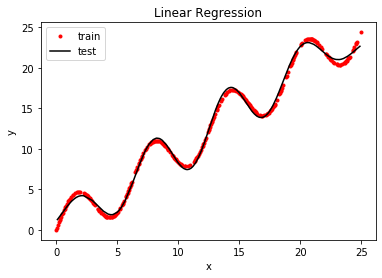
#显示结果
plt.plot(x_train, y_train, 'ro', markersize=3)
# plt.plot(x_test, y_test, 'k')
plt.plot(x_test, y_test_pred, 'k')
plt.xlabel('x')
plt.ylabel('y')
plt.title('Linear Regression')
plt.legend(['train', 'test', 'pred'])
plt.show()
运行结果:(调用identity_basis)
(300,)
(200,)
训练集预测值与真实值的标准差:2.0
预测值与真实值的标准差:2.1

运行结果:(调用multinomial_basis)
(300,)
(200,)
训练集预测值与真实值的标准差:2.0
预测值与真实值的标准差:2.2

运行结果:(调用gaussian_basis)
(300,)
(200,)
训练集预测值与真实值的标准差:0.4
预测值与真实值的标准差:0.4
linear_regression_tensorflow2.0
设计基函数(basis function) 以及数据读取
import numpy as np
import matplotlib.pyplot as plt

def identity_basis(x):
    ret = np.expand_dims(x, axis=1)
    return ret

def multinomial_basis(x, feature_num=10):
    x = np.expand_dims(x, axis=1) # shape(N, 1)
    feat = [x]
    for i in range(2, feature_num+1):
        feat.append(x**i)
    ret = np.concatenate(feat, axis=1)
    return ret

def gaussian_basis(x, feature_num=10):
    centers = np.linspace(0, 25, feature_num)
    width = 1.0 * (centers[1] - centers[0])
    x = np.expand_dims(x, axis=1)
    x = np.concatenate([x]*feature_num, axis=1)

    out = (x-centers)/width
    ret = np.exp(-0.5 * out ** 2)
    return ret

def load_data(filename, basis_func=gaussian_basis):
    """载入数据。"""
    xys = []
    with open(filename, 'r') as f:
        for line in f:
            xys.append(map(float, line.strip().split()))
        xs, ys = zip(*xys)
        xs, ys = np.asarray(xs), np.asarray(ys)

        o_x, o_y = xs, ys
        phi0 = np.expand_dims(np.ones_like(xs), axis=1)
        phi1 = basis_func(xs)
        xs = np.concatenate([phi0, phi1], axis=1)
        return (np.float32(xs), np.float32(ys)), (o_x, o_y)
定义模型
import tensorflow as tf
from tensorflow.keras import optimizers, layers, Model

class linearModel(Model):
    def __init__(self, ndim):
        super(linearModel, self).__init__()
        self.w = tf.Variable(
            shape=[ndim, 1],
            initial_value=tf.random.uniform(
                [ndim,1], minval=-0.1, maxval=0.1, dtype=tf.float32))

    @tf.function
    def call(self, x):
        y = tf.squeeze(tf.matmul(x, self.w), axis=1)
        return y

(xs, ys), (o_x, o_y) = load_data('train.txt')
ndim = xs.shape[1]

model = linearModel(ndim=ndim)
训练以及评估
optimizer = optimizers.Adam(0.1)
@tf.function
def train_one_step(model, xs, ys):
    with tf.GradientTape() as tape:
        y_preds = model(xs)
        loss = tf.reduce_mean(tf.sqrt(1e-12+(ys-y_preds)**2))
    grads = tape.gradient(loss, model.w)
    optimizer.apply_gradients([(grads, model.w)])
    return loss

@tf.function
def predict(model, xs):
    y_preds = model(xs)
    return y_preds

def evaluate(ys, ys_pred):
    """评估模型。"""
    std = np.sqrt(np.mean(np.abs(ys - ys_pred) ** 2))
    return std
for i in range(1000):
    loss = train_one_step(model, xs, ys)
    if i % 100 == 1:
        print(f'loss is {loss:.4}')


y_preds = predict(model, xs)
std = evaluate(ys, y_preds)
print('训练集预测值与真实值的标准差:{:.1f}'.format(std))

(xs_test, ys_test), (o_x_test, o_y_test) = load_data('test.txt')

y_test_preds = predict(model, xs_test)
std = evaluate(ys_test, y_test_preds)
print('训练集预测值与真实值的标准差:{:.1f}'.format(std))

plt.plot(o_x, o_y, 'ro', markersize=3)
plt.plot(o_x_test, y_test_preds, 'k')
plt.xlabel('x')
plt.ylabel('y')
plt.title('Linear Regression')
plt.legend(['train', 'test', 'pred'])
plt.show()
loss is 11.67
loss is 1.655
loss is 1.608
loss is 1.572
loss is 1.533
loss is 1.495
loss is 1.454
loss is 1.411
loss is 1.366
loss is 1.32
训练集预测值与真实值的标准差:1.5
训练集预测值与真实值的标准差:1.8
