笔记:Andrew Ng's Deeping Learning视频
参考:https://xienaoban.github.io/posts/41302.html
参考:https://blog.csdn.net/u012328159/article/details/80210363
1. 训练集、验证集、测试集(Train, Dev, Test Sets)
-
当数据量小的时候, 70% 训练, 30% 测试;或 60% 训练、20% 验证、20%测试.
-
训练集( training set):用来训练模型,即被用来 学习 得到系统的 参数取值.
-
测试集( testing set):用于最终报告模型的评价结果,因此在训练阶段测试集中的样本应该是不可见的.
-
对训练集做进一步划分为 训练集、验证集 validation set.
-
验证集:与测试集类似,也是用于评估模型的性能.
-
区别:是 验证集 主要 用于 模型选择 和 调整超参数,因而一般不用于报告最终结果.
-
-
-
当我们有大于100万条数据时, 测试集验证集各取1万条即可, 足以评估单个分类器.
-
确保验证集和测试集的数据来自同一分布.
-
如果不需要无偏估计, 可以不设置测试集; 当没设立测试集的时候, 验证集通常被人们称为测试集.
2. 偏差、方差(Bias, Variance)
-
高偏差(high bias)称为"欠拟合"(underfitting), 训练集误差与验证集误差都高.
- 选择一个新的网络,比如含有更多隐藏层或者隐藏单元的网络,或者花费更多时间来训练网络,或者尝试更先进的优化算法【后面深入讲解】
-
高方差(high variance)称为"过拟合"(overfitting), 训练集误差很低,而验证集误差很高.
-
解决方法是 正则化
-
准备更多的数据.
-


3. 正则化(Regularization)
- 避免过拟合
- 减少网络误差
3.1 逻辑回归中的L1正则化, L2正则化
对于L1正则化, 为代价函数添加L1范数:(几乎不用了)
其中:
- 使用L1正则化, w最终会是稀疏的(w中含很多0), 有利于压缩模型
- 但也没有降低太多内存, 所以不能将压缩作为L1正则化的目的。通常我们使用L2正则化.
对于L2正则化, 为代价函数添加L2范数:
其中:
尽管 (b) 也是参数, 但我们没有必要添加 (frac{lambda}{2m}b^2) 项, 因为 (w) 几乎涵盖了所有参数, 而 (b) 只是众多参数中的一个, 可以忽略不计(当然加上也没问题).
3.2 神经网络中的L2正则化
对于神经网络L2正则化(权重衰减),为代价函数添加L2范数:
其中,弗罗贝尼乌斯范数(即矩阵L2范数,矩阵中所有元素平方和):
则在反向传播时,
正则项说明, 无论 (w^{[l]}) 是什么, 我们都努力使之更小(趋于0), 则计算得的 (z^{[l]}=w^{[l]}a^{[l−1]}+b^{[l]}) 此时也更小
(z^{[l]}) 更容易(以tanh例) 落在激活函数 (g(z^{[l]})) 中间那一段接近线性的部分, 以达到简化网络的目的
- 注:线性的激活函数使得无论多少层的网络, 效果都和一层一样
3.3 随机失活(Dropout)正则化
对每一轮的训练, Dropout 遍历网络的每一层, 设置神经网络中每一层每个节点的失活概率
被随机选中失活的节点临时被消除, 不参与本轮的训练, 于是得到一个更小的网络.
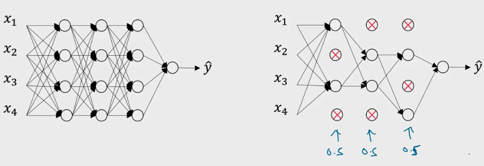
最常用的为反向随机失活(Inverted Dropout).
该方法在向前传播时, 根据随机失活的概率 (例如0.2),将每一层(例如 (l) 层)的 (a^{[l]}) 矩阵(a=g(z)) 中被选中失活的元素置为0, 则该层的 (a^{[l]}) 相当于少了 20% 的元素.
为了不影响下一层 (z^{[l+1]}) 的期望值, 我们需要 (a^{[l]}) /= 0.8 以修正权重.
代码实现:
- 前向传播
def forward_propagation_with_dropout(X, parameters, keep_prob = 0.8):
    """
    X -- input dataset, of shape (input size, number of examples)
    parameters -- python dictionary containing your parameters "W1", "b1", "W2", "b2",...,"WL", "bL"
                    W -- weight matrix of shape (size of current layer, size of previous layer)
                    b -- bias vector of shape (size of current layer,1)
    keep_prob: probability of keeping a neuron active during drop-out, scalar
    :return:
    AL: the output of the last Layer(y_predict)
    caches: list, every element is a tuple:(W,b,z,A_pre)
    """
    np.random.seed(1)  #random seed
    L = len(parameters) // 2            # number of layer
    A = X
    caches = [(None,None,None,X,None)]  # 用于存储每一层的,w,b,z,A,D第0层w,b,z用none代替
    # calculate from 1 to L-1 layer
    for l in range(1, L):
        A_pre = A
        W = parameters["W" + str(l)]
        b = parameters["b" + str(l)]
        z = np.dot(W, A_pre) + b  # 计算z = wx + b
        A = relu(z)  # relu activation function
        D = np.random.rand(A.shape[0], A.shape[1]) #initialize matrix D
        D = (D < keep_prob)       #convert entries of D to 0 or 1 (using keep_prob as the threshold)
        A = np.multiply(A, D)     #shut down some neurons of A
        A = A / keep_prob         # scale the value of neurons that haven't been shut down
        caches.append((W, b, z, A,D))
    # calculate Lth layer
    WL = parameters["W" + str(L)]
    bL = parameters["b" + str(L)]
    zL = np.dot(WL, A) + bL
    AL = sigmoid(zL)
    caches.append((WL, bL, zL, A))
    return AL, caches
- 后向传播
def backward_propagation_with_dropout(AL, Y, caches, keep_prob = 0.8):
    """
        Implement the backward propagation presented in figure 2.
        Arguments:
        X -- input dataset, of shape (input size, number of examples)
        Y -- true "label" vector (containing 0 if cat, 1 if non-cat)
        caches -- caches output from forward_propagation(),(W,b,z,pre_A)
        keep_prob: probability of keeping a neuron active during drop-out, scalar
        Returns:
        gradients -- A dictionary with the gradients with respect to dW,db
        """
    m = Y.shape[1]
    L = len(caches) - 1
    # print("L:   " + str(L))
    # calculate the Lth layer gradients
    prev_AL = caches[L - 1][3]
    dzL = 1. / m * (AL - Y)
    dWL = np.dot(dzL, prev_AL.T)
    dbL = np.sum(dzL, axis=1, keepdims=True)
    gradients = {"dW" + str(L): dWL, "db" + str(L): dbL}
    # calculate from L-1 to 1 layer gradients
    for l in reversed(range(1, L)): # L-1,L-2,...,1
        post_W = caches[l + 1][0]  # 要用后一层的W
        dz = dzL  # 用后一层的dz
        dal = np.dot(post_W.T, dz)
        Dl = caches[l][4] #当前层的D
        dal = np.multiply(dal, Dl) #Apply mask Dl to shut down the same neurons as during the forward propagation
        dal = dal / keep_prob #Scale the value of neurons that haven't been shut down
        Al = caches[l][3]  #当前层的A
        dzl = np.multiply(dal, relu_backward(Al))#也可以用dzl=np.multiply(dal, np.int64(Al > 0))来实现
        prev_A = caches[l-1][3]  # 前一层的A
        dWl = np.dot(dzl, prev_A.T)
        dbl = np.sum(dzl, axis=1, keepdims=True)

        gradients["dW" + str(l)] = dWl
        gradients["db" + str(l)] = dbl
        dzL = dzl  # 更新dz
    return gradients
注意:
-
训练时的 "(a^{[l]}) /= 0.8" 要修复权重
-
在测试阶段无需使用 Dropout.(测试阶段要关掉)
-
Dropout 不能与梯度检验同时使用,因为 Dropout 在梯度下降上的代价函数J难以计算.
3.4 其他正则化
数据扩增:
- 比如训练分类猫咪的图片, 将图片左右翻转、旋转一个小角度、稍微变形处理等, 可以人工合成数据.
Early Stopping:
-
运行梯度下降时, 我们可以绘制训练误差, 当验证集误差不降反增的时候, 停止训练.
-
缺点:是可能导致代价J值不够小, 却又没解决继续训练可能导致的过拟合问题.
4. 归一化(Normalizing)
- 加速训练
输入的归一化有两个步骤:
- 均值调整为0
- 方差归一化
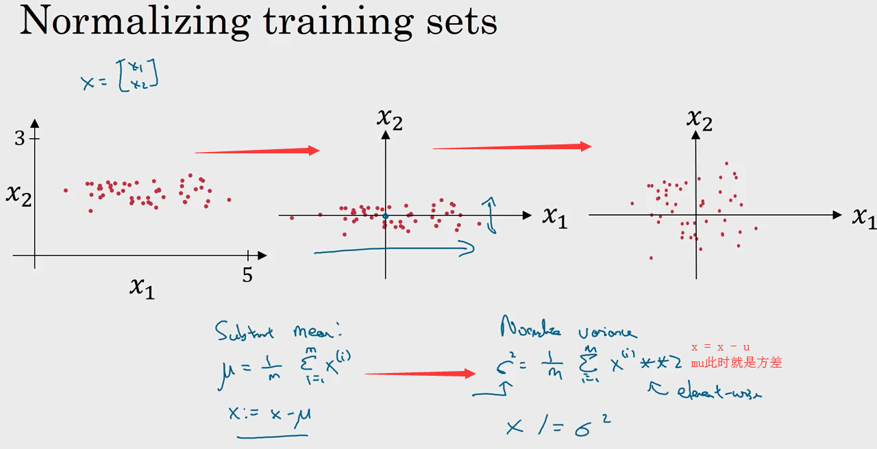
注:此时x1, x2方差均为1
归一化直观的理解就是使得代价函数更圆, 更容易优化代价函数.

5. 梯度消失/爆炸(Vanishing / Exploding Gradients)
- 加速训练
为了方便理解,假设使用了线性激活函数 g(z)=z , 且
则:
可知若 (W) 中有元素权重为 1.5 , 则最终得到 ({1.5}^{L−1}) 若层数很深, 计算得 (hat{y}) 也很大;
同理若权重为 0.5 , 进行 L−1 次幂运算后值会很小. 这便是梯度爆炸 与 梯度消失.
有效的解决方案:
-
由于 (z=w_1x_1+w_2x_2+...+w_nx_n) (忽略 (b)), 为了预防 (z) 太大或太小, 则 (n) 越大时, 期望 (w_i) 越小
-
则在随机(0~1)初始化 (W) 时, 我们对其乘上一个小于1的倍数, 使之更小.
-
对于Tanh, 权重乘上 (sqrt{frac{1}{n^{[l-1]}}}) 或者 (sqrt{frac{2}{n^{[l-1]}+n^{[l]}}})
-
对于Relu, 权重乘上 (sqrt{frac{2}{n^{[l-1]}}})
-
# GRADED FUNCTION: initialize_parameters_he

def initialize_parameters_he(layers_dims):
    """
    Arguments:
    layer_dims -- python array (list) containing the size of each layer.

    Returns:
    parameters -- python dictionary containing your parameters "W1", "b1", ..., "WL", "bL":
                    W1 -- weight matrix of shape (layers_dims[1], layers_dims[0])
                    b1 -- bias vector of shape (layers_dims[1], 1)
                    ...
                    WL -- weight matrix of shape (layers_dims[L], layers_dims[L-1])
                    bL -- bias vector of shape (layers_dims[L], 1)
    """

    np.random.seed(3)
    parameters = {}
    L = len(layers_dims) - 1 # integer representing the number of layers

    for l in range(1, L + 1):
        ### START CODE HERE ### (≈ 2 lines of code)
        parameters['W' + str(l)] = np.random.randn(layers_dims[l], layers_dims[l-1]) * (np.sqrt(2. / layers_dims[l-1]))
        parameters['b' + str(l)] = np.zeros((layers_dims[l], 1))
        ### END CODE HERE ###

    return parameters
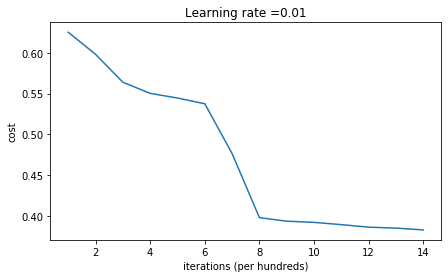
随机用大的数进行初始化W,画出的cost下降的曲线:
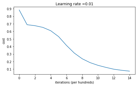
用上面方法进行初始化W,画出的cost下降的曲线:
6. 梯度检验
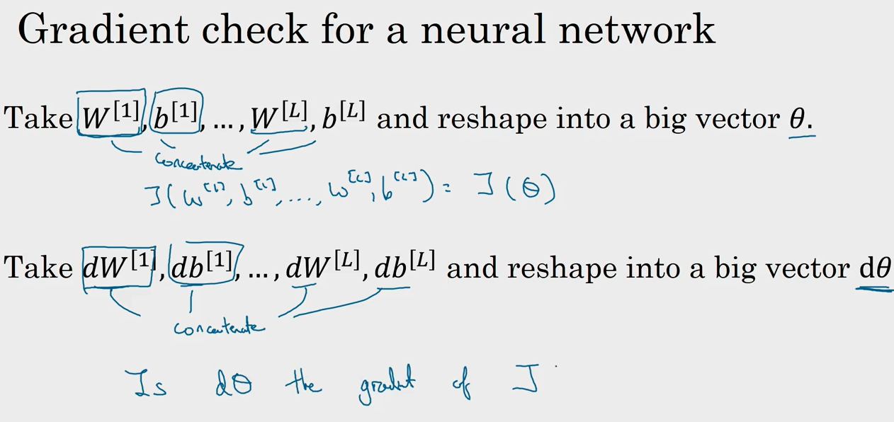
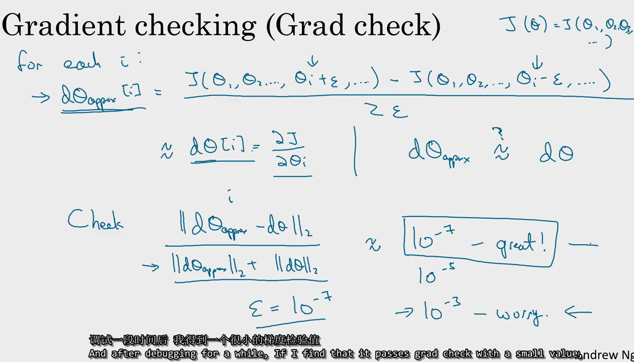
在反向传播的时候, 如果怕自己 (d heta[i] = frac{partial J}{partial heta_i}) 等算错, 可以用导数的定义, 计算
({for each i:})
然后根据 两者误差 估计自己是否算错. 该方法仅用来调试
且不能同 Dropout 同时使用.