为了实现某些运算,需要快速构造符合要求的大数组
Numpy函数生成的数组,如不指定类类型,几乎全为浮点型(arange除外,它是整形),因为科学计算中测量值,例如温度、长度,都是浮点数
1 import numpy as np
2 import matplotlib.pyplot as plt
3 plt.style.use('seaborn')
1 np.arange(20)
array([ 0,  1,  2,  3,  4,  5,  6,  7,  8,  9, 10, 11, 12, 13, 14, 15, 16,
       17, 18, 19])
1 np.arange(5,15)
array([ 5, 6, 7, 8, 9, 10, 11, 12, 13, 14])
1 np.arange(5,15,2) # 起始,终点,步长
array([ 5, 7, 9, 11, 13])
1 np.linspace(1,10,4)
array([ 1., 4., 7., 10.])
1 np.linspace(1,10,4,endpoint=False) #endpoint表示终止元素是否是n个生成元素中的一个
array([1. , 3.25, 5.5 , 7.75])
1 # 作为参数的数组
2 n1 = np.array([[1,2,3],[4,5,6]])
3 n1
array([[1, 2, 3],
       [4, 5, 6]])
1 np.ones(10)
array([1., 1., 1., 1., 1., 1., 1., 1., 1., 1.])
1 np.ones((3,5))
array([[1., 1., 1., 1., 1.],
       [1., 1., 1., 1., 1.],
       [1., 1., 1., 1., 1.]])
1 np.ones((3,5,2))
array([[[1., 1.],
        [1., 1.],
        [1., 1.],
        [1., 1.],
        [1., 1.]],

       [[1., 1.],
        [1., 1.],
        [1., 1.],
        [1., 1.],
        [1., 1.]],

       [[1., 1.],
        [1., 1.],
        [1., 1.],
        [1., 1.],
        [1., 1.]]])
1 np.ones_like(n1)
array([[1, 1, 1],
       [1, 1, 1]])
1 np.zeros(5)
array([0., 0., 0., 0., 0.])
1 np.zeros((3,5))
array([[0., 0., 0., 0., 0.],
       [0., 0., 0., 0., 0.],
       [0., 0., 0., 0., 0.]])
1 np.zeros((3,5),dtype=np.int)
array([[0, 0, 0, 0, 0],
       [0, 0, 0, 0, 0],
       [0, 0, 0, 0, 0]])
1 np.zeros_like(n1)
array([[0, 0, 0],
       [0, 0, 0]])
1 np.empty(5)
array([0., 0., 0., 0., 0.])
1 np.empty((3,5))
array([[0., 0., 0., 0., 0.],
       [0., 0., 0., 0., 0.],
       [0., 0., 0., 0., 0.]])
1 np.empty_like(n1)
array([[1761607734,        627,     159849],
       [  15198464, 1986592768, 1761607682]])
1 np.full(10,33)
array([33, 33, 33, 33, 33, 33, 33, 33, 33, 33])
1 np.full((3,2),33)
array([[33, 33],
       [33, 33],
       [33, 33]])
1 np.full_like(n1,33)
array([[33, 33, 33],
       [33, 33, 33]])
1 # n * n 矩阵,对角线为1,其余为0
2 np.eye(5)
array([[1., 0., 0., 0., 0.],
       [0., 1., 0., 0., 0.],
       [0., 0., 1., 0., 0.],
       [0., 0., 0., 1., 0.],
       [0., 0., 0., 0., 1.]])
1 np.identity(5)
array([[1., 0., 0., 0., 0.],
       [0., 1., 0., 0., 0.],
       [0., 0., 1., 0., 0.],
       [0., 0., 0., 1., 0.],
       [0., 0., 0., 0., 1.]])
1 #正方形矩阵
2 np.diag([1,3,5,7,9])
array([[1, 0, 0, 0, 0],
       [0, 3, 0, 0, 0],
       [0, 0, 5, 0, 0],
       [0, 0, 0, 7, 0],
       [0, 0, 0, 0, 9]])
使用Numpy随机数创建特定数组
数值模拟和可视化经常需要生成各种随机数数组
np.random随机数子库对py内置random进行了补充
均匀分布随机数
1 # 均匀分布随机数
2 np.random.rand(10) #给定维度
array([0.02005439, 0.80891558, 0.5562677 , 0.46869316, 0.92231742,
       0.48360549, 0.60707295, 0.8765322 , 0.03622524, 0.56985785])
1 np.random.rand(3,4,5) #给定维度
array([[[0.72599464, 0.83993961, 0.82219185, 0.82398166, 0.36356688],
        [0.39168192, 0.30798546, 0.44759764, 0.1118108 , 0.85378293],
        [0.82600419, 0.32026777, 0.21802031, 0.36702474, 0.97069152],
        [0.33273498, 0.99248325, 0.11253019, 0.18952265, 0.86363985]],

       [[0.79576536, 0.84591304, 0.51058729, 0.17913884, 0.33642013],
        [0.73720407, 0.177351  , 0.95445729, 0.95058418, 0.6877008 ],
        [0.54047611, 0.40272865, 0.57165086, 0.40991547, 0.88575988],
        [0.99419175, 0.78947254, 0.73026638, 0.11067003, 0.97844173]],

       [[0.06063713, 0.19173863, 0.72189927, 0.87016215, 0.79903106],
        [0.490451  , 0.22794955, 0.24318515, 0.79332367, 0.98940884],
        [0.64366935, 0.78009235, 0.91986054, 0.91137557, 0.8464019 ],
        [0.93800903, 0.79523183, 0.27570733, 0.91195909, 0.65208651]]])
1 # 绘图测试
2 a = np.random.rand(500) #给定维度
3 plt.hist(
4     a,
5     facecolor = '#cccccc', #直方图颜色
6     edgecolor = 'w', #直方图边框颜色
7 )
8 plt.show()

1 #均匀分布,带起始,结束值
2 np.random.uniform(5,10,20)
array([8.69273352, 9.74400917, 9.63900495, 8.13481997, 9.37227264,
       8.19094361, 5.90780594, 6.87353705, 5.13186801, 5.20761676,
       7.80789903, 7.77578052, 7.8747056 , 8.32116957, 9.05401958,
       7.99650407, 8.21572178, 9.84023002, 6.45075345, 6.28031921])
1 np.random.uniform(5,10,(3,5))
array([[8.15258875, 9.46890301, 6.87993789, 9.67530067, 7.71837652],
       [8.33403327, 5.67919505, 7.00191982, 7.09070637, 8.21504323],
       [5.69171455, 7.14411578, 6.03591799, 8.96227029, 6.27297609]])
1 #均匀分布,整数
2 np.random.randint(10)
1
1 np.random.randint(10,100)
77
1 np.random.randint(10,20,(3,4,5))
array([[[14, 15, 13, 19, 17],
        [13, 17, 10, 12, 18],
        [18, 19, 17, 18, 10],
        [17, 15, 18, 16, 14]],

       [[11, 17, 16, 11, 14],
        [15, 11, 17, 16, 18],
        [18, 13, 15, 18, 19],
        [10, 17, 18, 10, 14]],

       [[10, 14, 18, 14, 10],
        [11, 14, 18, 19, 16],
        [16, 16, 12, 12, 16],
        [13, 16, 14, 16, 12]]])
随机数种子
相同的种子,相同的随机数
1 np.random.seed(1)
2 np.random.rand(10)
array([4.17022005e-01, 7.20324493e-01, 1.14374817e-04, 3.02332573e-01,
       1.46755891e-01, 9.23385948e-02, 1.86260211e-01, 3.45560727e-01,
       3.96767474e-01, 5.38816734e-01])
1 np.random.seed(1)
2 np.random.rand(10)
array([4.17022005e-01, 7.20324493e-01, 1.14374817e-04, 3.02332573e-01,
       1.46755891e-01, 9.23385948e-02, 1.86260211e-01, 3.45560727e-01,
       3.96767474e-01, 5.38816734e-01])
正态分布
1 #标准正太分布随机数,浮点数,平局数0,标准差1
2 np.random.randn(10)
array([-1.11731035,  0.2344157 ,  1.65980218,  0.74204416, -0.19183555,
       -0.88762896, -0.74715829,  1.6924546 ,  0.05080775, -0.63699565])
1 np.random.randn(3,4,5)
array([[[ 0.19091548,  2.10025514,  0.12015895,  0.61720311,
          0.30017032],
        [-0.35224985, -1.1425182 , -0.34934272, -0.20889423,
          0.58662319],
        [ 0.83898341,  0.93110208,  0.28558733,  0.88514116,
         -0.75439794],
        [ 1.25286816,  0.51292982, -0.29809284,  0.48851815,
         -0.07557171]],

       [[ 1.13162939,  1.51981682,  2.18557541, -1.39649634,
         -1.44411381],
        [-0.50446586,  0.16003707,  0.87616892,  0.31563495,
         -2.02220122],
        [-0.30620401,  0.82797464,  0.23009474,  0.76201118,
         -0.22232814],
        [-0.20075807,  0.18656139,  0.41005165,  0.19829972,
          0.11900865]],

       [[-0.67066229,  0.37756379,  0.12182127,  1.12948391,
          1.19891788],
        [ 0.18515642, -0.37528495, -0.63873041,  0.42349435,
          0.07734007],
        [-0.34385368,  0.04359686, -0.62000084,  0.69803203,
         -0.44712856],
        [ 1.2245077 ,  0.40349164,  0.59357852, -1.09491185,
          0.16938243]]])
1 #绘图
2 b = np.random.randn(500)
3 plt.hist(
4     b,
5     facecolor='#cccccc',#直方图颜色
6     edgecolor='w',#直方图边框颜色
7 )
8 plt.show()
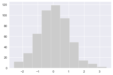
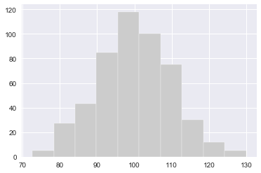
1 # 自定义正态分布,分布中心是loc(概率分布的均值),标准差是scale,形状是size
2 np.random.normal(100,10,500)
3 np.random.normal(100,10,(3,4,5))
4 plt.hist(
5     np.random.normal(100,10,500),
6     facecolor='#cccccc',#直方图颜色
7     edgecolor='w',#直方图边框颜色
8 )
9 plt.show()
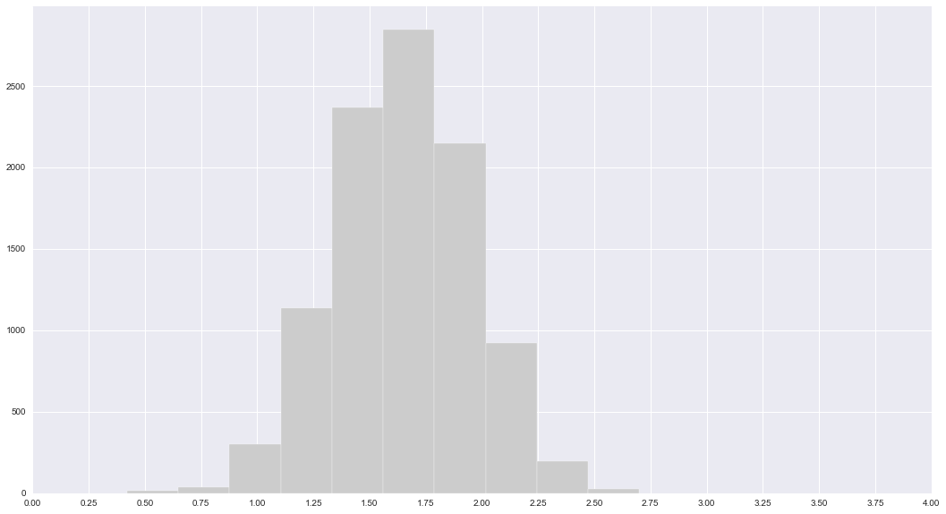
案例:中国成年男性身高分析
生成男性身高数据
1 # 均与分布不符合现实
2 # height = np.round(np.random.uniform(1.1,2.4,500),2)
3
4 #自定义正态分布,均值1.67,标准差0.3 生成10000个,保留2位小数
5 height = np.round(np.random.normal(1.65,0.3,10000),2)
6 height
array([1.26, 1.75, 1.69, ..., 1.55, 1.49, 1.62])
1 plt.figure(figsize=(18,10))
2 plt.hist(
3     height,
4     facecolor='#cccccc', #直方图颜色
5     edgecolor = 'w' , #直方图边框颜色
6 )
7 plt.xticks([0,0.25,0.5,0.75,1,1.25,1.5,1.75,2,2.25,2.5,2.75,3,3.25,3.5,3.75,4])
8 plt.show()
1 y = np.array([-2,3,-3,4])
2 x = [1,2,3,4]
3 plt.bar(x,y)
4 plt.show()

1 np.log
<ufunc 'log'>
1 10 ** 2
100
1 np.log2(1/32)
-5.0