前言
理论知识:UFLDL教程和http://www.cnblogs.com/tornadomeet/archive/2013/04/09/3009830.html
实验环境:win7, matlab2015b,16G内存,2T机械硬盘
实验内容:Exercise:Convolution and Pooling。从2000张64*64的RGB图片(它是 the STL10 Dataset的一个子集)中提取特征作为训练数据集,训练softmax分类器,然后从3200张64*64的RGB图片(它是 the STL10 Dataset的另一个子集)中提取特征作为测试数据集,输入到前面已经训练好的softmax分类器,把这3200张图片分为4类:airplane, car, cat, dog。
实验基础说明:
1.怎么样从2000张64*64的RGB图片中提取特征得到训练集,怎么样从3200张64*64的RGB图片中提取特征得到测试集?
因为这里的RGB图片是64*64,尺寸较大,而不是前面所有实验中用的8*8的小图像块,如果用Deep Learning九之深度学习UFLDL教程:linear decoder_exercise(斯坦福大学深度学习教程)中的方法直接从大尺寸图片中提取特征,那么运算量就太大,所以,为了减小运算量,不能直接从大尺寸图片中提取特征,而是要用间接的减小运算量的方法,这个方法利用了自然图像的固有特性:自然图像的一部分的统计特性与其他部分是一样的。这个固有特性也就意味着:从自然图像的某一部分A中学习的特征L_feature也能用在该自然图像的另一部分B上。也就是说,对于这个自然图像上的所有位置,我们都能使用同样的学习特征。那么究竟怎么样从这个大尺寸自然图像提取出它的L_feature特征呢(这个特征是从它的一部分A上学习到的)?答案是卷积!即把这个特征和大尺寸图片相卷,就可以提取这个大尺寸图片的L_feature特征,至于原因请看下面。这个L_feature特征维数只会比大尺寸图片稍微小一点(假设从小图像块中学习到的特征是8*8,大尺寸图片是64*64,那么这个L_feature特征就是(64-8+1)*(64-8+1),即:57*57),如果把这些特征作训练数据集,那么运算量还是很大,输入层神经元节点数还是要57*57*3个,所以我们再对这些特征用池化的方法(即:假设池化的维数是19,池化就是把57*57的特征依次分为19*19的9个小部分,然后把每个小部分变为一个值(如果这个值是每个小部分的平均值就是平均池化,是最大值就是最大池化),从而把这个57*57的特征变为了3*3的特征),从而最后从2000张64*64的RGB图片中提取出了3*3的特征得到了训练数据集,同理,可得到测试数据集。
具体方法:
①是从the STL10 Dataset中随机抽样选出10万张8*8的RGB小图像块(即:Sampled 8x8 patches from the STL-10 dataset),然后对它们进行预处理,具体包括:先对它们进行0均值化(注意:不是每个样本各自单独0均值化),再对它们进行ZCA白化。
②是对预处理后的数据利用线性解码器提取出M个颜色特征。
前两步已经在Deep Learning九之深度学习UFLDL教程:linear decoder_exercise(斯坦福大学深度学习教程)中实现。
③是把2000张64*64的 RGB图片中的每一张图片都分别与第二步中提取出的M个特征相卷积,从而就能在每张64*64的 RGB图片中都提取出在第二步中学习到的M个特征,共得到2000*M个卷积特征。
④是把这2000*M个特征进行池化,减小它的维数,从而得到了训练数据集。同理,可得到测试数据集。
后两步就是本节实验的内容。
2.为什么从自然图像上的一部分A提取出L_feature特征后,要提取这整张自然图像的L_feature特征的方法是:把这个特征和这个自然图像相卷积?
首先,我们要明确知道:
① 卷积运算图解:

② 从数据集Y中提取特征F(F是从数据集X中通过稀疏自动编码器提取到的特征)的方法:
如果用数据集X训练稀疏自动编码器,得到稀疏自动编码器的权重参数是opttheta,从而就提取到特征F,F就是稀疏自动编码器的激活值,即F=sigmod(X*opttheta),而把数据集Y通过该训练过稀疏自动编码器得到的激活值就是从数据集Y中提取的特征F,即:F=sigmod(Y*opttheta)。
这一点实际上已经在Deep Learning七之深度学习UFLDL教程:Self-Taught Learning_Exercise(斯坦福大学深度学习教程)的“实验内容及步骤”中的第一、二点提到。
③ 我们要清楚从自然图像的某一部分A中提取L_feature特征的方法是线性解码器,它的第一层实际上是一个稀疏自动编码器(假设用A来训练该稀疏自动编码器得到其网络参数为opttheta1),我们说的这个L_feature特征实际上就是这个第一层稀疏自动编码器的激活值,即:L_feature=sigmod(A*opttheta1)。
其次,在清楚以上三点的情况下,我们才能进行如下说明:
假设这个L_feature特征大小是8*8,要从这整张自然图像中提取L_feature特征的方法是:从这整张自然图像上依次抽取8*8区域Q通过前面提到的网络参数为opttheta1的稀疏自动编码器,即可得到从Q上提取的L_feature特征,即为其激活值:L_feature=sigmod(Q*opttheta1)。这些所有8*8区域提取的L_feature特征组合在一起,就是这整张自然图像上提取的L_feature特征。这个过程就是Ng在讲解中说明的,把这个L_feature特征作为探测器,应用到这个图像的任意地方中去的过程。这个过程如下:

而这以上整个过程,基本正好符合卷积运算,所以我们把得到特征叫卷积特征,即:这个过程基本正好是opttheta1与整张自然图像的卷积过程,只两个不同之处:
a. 卷积运算时,opttheta1的倒序依次与区域Q相乘,而我们实际计算L_feature特征时opttheta1不是倒序的。所以为了能直接运用卷积,我们可先把opttheta1倒序再与整张自然图像进行卷积,得到的就正好是L_feature特征。所以,在cnnConvolve.m中的cnnConvolve函数有这句代码来倒序:
feature = rot90(squeeze(feature),2);
当然,Ng用的是这句:
feature = flipud(fliplr(squeeze(feature)));
相比起来, rot90的运行速度更快,我在这里做了改进。
b. 整个卷积运算过程实际上还包含了使用边缘补 0 部分进行计算的卷积结果部分,而我们并不需要这个部分,所以我们在cnnConvolve.m中的cnnConvolve函数中有:
convolvedImage = convolvedImage + conv2(im, feature, 'valid');
参数valid使返回在卷积过程中,未使用边缘补 0 部分进行计算的卷积结果部分。
综上,所以把这个特征和这个自然图像相卷积即可提取这整张自然图像的L_feature特征。
3.一些matlab函数
squeeze: 移除单一维
使用方法 :B=squeeze(A)
返回和矩阵A相同元素但所有单一维都移除的矩阵B,单一维是满足size(A,dim)=1的维。
squeeze命令对二维数组是不起作用的;
如果A是一行或列向量或一标量(1*1)值,则B=A。
例如:2*1*3 数组Y = rand(2,1,3). 这个数组有单一维 —就是每页仅仅一列:
Y =
Y(:,:,1) =
0.5194
0.8310
Y(:,:,2) =
0.0346
0.0535
Y(:,:,3) =
0.5297
0.6711
命令Z = squeeze(Y)结果是2*3矩阵:
Z =
0.5194 0.0346 0.5297
0.8310 0.0535 0.6711
rot90(X)
Ng教程中用的是:W = flipud(fliplr(W));
这个函数可用rot90(W,2)代替,因为它的运行速度更快。估计是Ng写这个教程的时候在2011年,rot90这个函数在matlab中还没出现,好像是在2012年才出现的。
用法:rot90(X),其中X表示一个矩阵。
功能:rot90函数是matlab中使一个矩阵逆时针旋转90度的函数。Y=rot90(X)表示使矩阵X逆时针旋转90度,作为新的矩阵Y,但矩阵X本身不变。
rot90(x,2),其中X表示一个矩阵。功能:将矩阵x旋转180度,形成新的矩阵,但x本身不变。
rot90(x,n),其中x表示一个矩阵,n为正整数,默认功能:将矩阵x逆时针旋转90*n度,形成新矩阵,x本身不变。
conv2
格式:C=conv2(A,B)
C=conv2(Hcol,Hrow,A)
C=conv2(...,'shape')
说明:
C=conv2(A,B) ,conv2 的算矩阵 A 和 B 的卷积,若 [Ma,Na]=size(A), [Mb,Nb]=size(B), 则 size(C)=[Ma+Mb-1,Na+Nb-1];
C=conv2(Hcol,Hrow,A) 中,矩阵 A 分别与 Hcol 向量在列方向和 Hrow 向量在行方向上进行卷积;
C=conv2(...,'shape') 用来指定 conv2返回二维卷积结果部分,参数 shape 可取值如下:
full 为缺省值,返回二维卷积的全部结果;
same 返回二维卷积结果中与 A 大小相同的中间部分;
valid 返回在卷积过程中,未使用边缘补 0 部分进行计算的卷积结果部分,当 size(A)>size(B)时,size(C)=[Ma-Mb+1,Na-Nb+1]
permute
语法格式:
B = permute(A,order)
按照向量order指定的顺序重排A的各维。B中元素和A中元素完全相同。但由于经过重新排列,在A、B访问同一个元素使用的下标就不一样了。order中的元素必须各不相同
三维:
a=rand(2,3,4); %这是一个三维数组,各维的长度分别为:2,3,4
%现在交换第一维和第二维:
permute(A,[2,1,3]) %变成3*2*4的矩阵
二维:
二维的更形象,a=[1,2+j;3+2*j,4+5*j];permute(a,[2,1]),相当于把行(x)、列(y)互换;有别于转置(a'),你试一下就知道了。所以就叫非共轭转置。
4.优秀的编程技巧:
①在Ng的代码中,总是有检查的习惯,无论是前面的梯度计算还是本节实验中的卷积和池化等,Ng都会在计算完后想办法来验证前面的计算是否正确,这是一个良好的习惯,起码可以保证这些关键步骤没有错误。
②可用类似语句来检查代码:
assert(mod(hiddenSize, stepSize) == 0, 'stepSize should divide hiddenSize');
以及
if abs(features(featureNum, 1) - convolvedFeatures(featureNum, imageNum, imageRow, imageCol)) > 1e-9
fprintf('Convolved feature does not match activation from autoencoder
');
end
5.
代价函数  为:
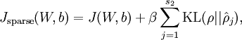
为:
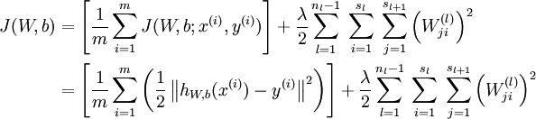
 ,其中
,其中 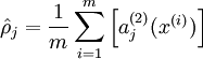
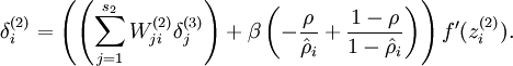
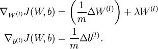
计算梯度需要用到的公式:
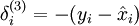 ,其中y是期望的输出。
 其中,
其中, 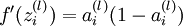
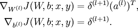
令  ,
, 


疑问
1.从代码中可看出,为什么对10万张小图像块要经过预处理(0均值化和ZCA白化),而对2000张和3200张64*64RGB图片却未进行预处理?感觉自己对什么时候该进行预处理,什么时候不用进行预处理,为什么这样,都没完全掌握!比如:在Deep Learning四之深度学习UFLDL教程:PCA in 2D_Exercise(斯坦福大学深度学习教程)中为什么二维数据不用进行0均值化,而自然图像就要先0均值化?
实验步骤
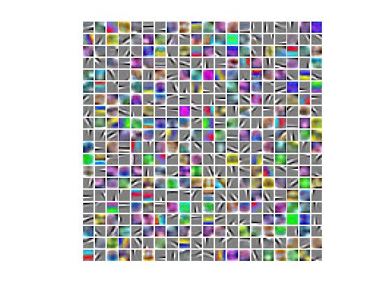
1.初始化参数,加载上一节实验结果,即:10万张8*8的RGB小图像块中提取的颜色特征,并把特征可视化。
2.先加载8张64*64的图片(用来测试卷积和池化是否正确),再实现卷积函数cnnConvolve.m,并检查该函数是否正确。
3.实现池化函数cnnPool.m,并检查该函数是否正确。
4.加载2000张64*64RGB图片,利用前面实现的卷积函数从中提取出卷积特征convolvedFeaturesThis后,再利用池化函数从convolvedFeaturesThis中提取出池化特征pooledFeaturesTrain,把它作为softmax分类器的训练数据集;加载3200张64*64RGB图片,利用前面实现的卷积函数从中提取出卷积特征convolvedFeaturesThis后,再利用池化函数从convolvedFeaturesThis中提取出池化特征pooledFeaturesTest,把它作为softmax分类器的测试数据集。
5.用训练数据集pooledFeaturesTrain及其标签训练softmax分类器,得到模型参数softmaxModel。
6.利用训练过的模型参数为pooledFeaturesTest的softmax分类器对测试数据集pooledFeaturesTest进行分类,即得到3200张64*64RGB图片的分类结果。
运行结果
Accuracy: 80.313%
所有训练数据和测试数据的卷积和池化特征的提取所用时间为:
Elapsed time is 2644.920372 seconds.
特征可视化结果:
代码
cnnExercise.m
%% CS294A/CS294W Convolutional Neural Networks Exercise

%  Instructions
%  ------------
%
%  This file contains code that helps you get started on the
%  convolutional neural networks exercise. In this exercise, you will only
%  need to modify cnnConvolve.m and cnnPool.m. You will not need to modify
%  this file.

%%======================================================================
%% STEP 0: Initialization
%  Here we initialize some parameters used for the exercise.

imageDim = 64;         % image dimension
imageChannels = 3;     % number of channels (rgb, so 3)

patchDim = 8;          % patch dimension
numPatches = 50000;    % number of patches

visibleSize = patchDim * patchDim * imageChannels;  % number of input units
outputSize = visibleSize;   % number of output units
hiddenSize = 400;           % number of hidden units

epsilon = 0.1;           % epsilon for ZCA whitening

poolDim = 19;          % dimension of pooling region

%%======================================================================
%% STEP 1: Train a sparse autoencoder (with a linear decoder) to learn
%  features from color patches. If you have completed the linear decoder
%  execise, use the features that you have obtained from that exercise,
%  loading them into optTheta. Recall that we have to keep around the
%  parameters used in whitening (i.e., the ZCA whitening matrix and the
%  meanPatch)

% --------------------------- YOUR CODE HERE --------------------------
% Train the sparse autoencoder and fill the following variables with
% the optimal parameters:

optTheta =  zeros(2*hiddenSize*visibleSize+hiddenSize+visibleSize, 1);
ZCAWhite =  zeros(visibleSize, visibleSize);
meanPatch = zeros(visibleSize, 1);
load STL10Features.mat;

% --------------------------------------------------------------------

% Display and check to see that the features look good
W = reshape(optTheta(1:visibleSize * hiddenSize), hiddenSize, visibleSize);
b = optTheta(2*hiddenSize*visibleSize+1:2*hiddenSize*visibleSize+hiddenSize);

displayColorNetwork( (W*ZCAWhite)');

%%======================================================================
%% STEP 2: Implement and test convolution and pooling
%  In this step, you will implement convolution and pooling, and test them
%  on a small part of the data set to ensure that you have implemented
%  these two functions correctly. In the next step, you will actually
%  convolve and pool the features with the STL10 images.

%% STEP 2a: Implement convolution
%  Implement convolution in the function cnnConvolve in cnnConvolve.m

% Note that we have to preprocess the images in the exact same way
% we preprocessed the patches before we can obtain the feature activations.

load stlTrainSubset.mat % loads numTrainImages, trainImages, trainLabels

%% 只用8张图片来测试卷积和池化是否正确 Use only the first 8 images for testing
convImages = trainImages(:, :, :, 1:8);  % 格式:trainImages(r, c, channel, image number)

% NOTE: Implement cnnConvolve in cnnConvolve.m first!
convolvedFeatures = cnnConvolve(patchDim, hiddenSize, convImages, W, b, ZCAWhite, meanPatch);

%% STEP 2b: Checking your convolution
%  To ensure that you have convolved the features correctly, we have
%  provided some code to compare the results of your convolution with
%  activations from the sparse autoencoder

% For 1000 random points
for i = 1:1000
    featureNum = randi([1, hiddenSize]);
    imageNum = randi([1, 8]);
    imageRow = randi([1, imageDim - patchDim + 1]);
    imageCol = randi([1, imageDim - patchDim + 1]);

    patch = convImages(imageRow:imageRow + patchDim - 1, imageCol:imageCol + patchDim - 1, :, imageNum);
    patch = patch(:);  % 将patch矩阵从3维矩阵转换为一个列向量
    patch = patch - meanPatch;
    patch = ZCAWhite * patch;  % 白化后的数据

    features = feedForwardAutoencoder(optTheta, hiddenSize, visibleSize, patch);

    if abs(features(featureNum, 1) - convolvedFeatures(featureNum, imageNum, imageRow, imageCol)) > 1e-9
        fprintf('Convolved feature does not match activation from autoencoder
');
        fprintf('Feature Number    : %d
', featureNum);
        fprintf('Image Number      : %d
', imageNum);
        fprintf('Image Row         : %d
', imageRow);
        fprintf('Image Column      : %d
', imageCol);
        fprintf('Convolved feature : %0.5f
', convolvedFeatures(featureNum, imageNum, imageRow, imageCol));
        fprintf('Sparse AE feature : %0.5f
', features(featureNum, 1));
        error('Convolved feature does not match activation from autoencoder');
    end
end

disp('Congratulations! Your convolution code passed the test.');

%% STEP 2c: Implement pooling
%  Implement pooling in the function cnnPool in cnnPool.m

% NOTE: Implement cnnPool in cnnPool.m first!
pooledFeatures = cnnPool(poolDim, convolvedFeatures);

%% STEP 2d: Checking your pooling
%  To ensure that you have implemented pooling, we will use your pooling
%  function to pool over a test matrix and check the results.

testMatrix = reshape(1:64, 8, 8);
expectedMatrix = [mean(mean(testMatrix(1:4, 1:4))) mean(mean(testMatrix(1:4, 5:8))); ...
                  mean(mean(testMatrix(5:8, 1:4))) mean(mean(testMatrix(5:8, 5:8))); ];

testMatrix = reshape(testMatrix, 1, 1, 8, 8);

pooledFeatures = squeeze(cnnPool(4, testMatrix));

if ~isequal(pooledFeatures, expectedMatrix)
    disp('Pooling incorrect');
    disp('Expected');
    disp(expectedMatrix);
    disp('Got');
    disp(pooledFeatures);
else
    disp('Congratulations! Your pooling code passed the test.');
end

%%======================================================================
%% STEP 3: Convolve and pool with the dataset
%  In this step, you will convolve each of the features you learned with
%  the full large images to obtain the convolved features. You will then
%  pool the convolved features to obtain the pooled features for
%  classification.
%
%  Because the convolved features matrix is very large, we will do the
%  convolution and pooling 50 features at a time to avoid running out of
%  memory. Reduce this number if necessary

stepSize = 50;
assert(mod(hiddenSize, stepSize) == 0, 'stepSize should divide hiddenSize');

load stlTrainSubset.mat % loads numTrainImages, trainImages, trainLabels
load stlTestSubset.mat  % loads numTestImages,  testImages,  testLabels

pooledFeaturesTrain = zeros(hiddenSize, numTrainImages, ...
    floor((imageDim - patchDim + 1) / poolDim), ...
    floor((imageDim - patchDim + 1) / poolDim) );
pooledFeaturesTest = zeros(hiddenSize, numTestImages, ...
    floor((imageDim - patchDim + 1) / poolDim), ...
    floor((imageDim - patchDim + 1) / poolDim) );

tic();

for convPart = 1:(hiddenSize / stepSize)

    featureStart = (convPart - 1) * stepSize + 1;
    featureEnd = convPart * stepSize;

    fprintf('Step %d: features %d to %d
', convPart, featureStart, featureEnd);
    Wt = W(featureStart:featureEnd, :);
    bt = b(featureStart:featureEnd);

    fprintf('Convolving and pooling train images
');
    convolvedFeaturesThis = cnnConvolve(patchDim, stepSize, ...
        trainImages, Wt, bt, ZCAWhite, meanPatch);
    pooledFeaturesThis = cnnPool(poolDim, convolvedFeaturesThis);
    pooledFeaturesTrain(featureStart:featureEnd, :, :, :) = pooledFeaturesThis;
    toc();
    clear convolvedFeaturesThis pooledFeaturesThis;

    fprintf('Convolving and pooling test images
');
    convolvedFeaturesThis = cnnConvolve(patchDim, stepSize, ...
        testImages, Wt, bt, ZCAWhite, meanPatch);
    pooledFeaturesThis = cnnPool(poolDim, convolvedFeaturesThis);
    pooledFeaturesTest(featureStart:featureEnd, :, :, :) = pooledFeaturesThis;
    toc();

    clear convolvedFeaturesThis pooledFeaturesThis;

end


% You might want to save the pooled features since convolution and pooling takes a long time
save('cnnPooledFeatures.mat', 'pooledFeaturesTrain', 'pooledFeaturesTest');
toc();

%%======================================================================
%% STEP 4: Use pooled features for classification
%  Now, you will use your pooled features to train a softmax classifier,
%  using softmaxTrain from the softmax exercise.
%  Training the softmax classifer for 1000 iterations should take less than
%  10 minutes.

% Add the path to your softmax solution, if necessary
% addpath /path/to/solution/

% Setup parameters for softmax
softmaxLambda = 1e-4;
numClasses = 4;
% Reshape the pooledFeatures to form an input vector for softmax
softmaxX = permute(pooledFeaturesTrain, [1 3 4 2]); % 把pooledFeaturesTrain的第2维移到最后
softmaxX = reshape(softmaxX, numel(pooledFeaturesTrain) / numTrainImages,...
    numTrainImages);
softmaxY = trainLabels;

options = struct;
options.maxIter = 200;
softmaxModel = softmaxTrain(numel(pooledFeaturesTrain) / numTrainImages,...
    numClasses, softmaxLambda, softmaxX, softmaxY, options);

%%======================================================================
%% STEP 5: Test classifer
%  Now you will test your trained classifer against the test images

softmaxX = permute(pooledFeaturesTest, [1 3 4 2]);
softmaxX = reshape(softmaxX, numel(pooledFeaturesTest) / numTestImages, numTestImages);
softmaxY = testLabels;

[pred] = softmaxPredict(softmaxModel, softmaxX);
acc = (pred(:) == softmaxY(:));
acc = sum(acc) / size(acc, 1);
fprintf('Accuracy: %2.3f%%
', acc * 100);

% You should expect to get an accuracy of around 80% on the test images.
cnnConvolve.m
function convolvedFeatures = cnnConvolve(patchDim, numFeatures, images, W, b, ZCAWhite, meanPatch)
%卷积特征提取:把每一个特征都与每一张大尺寸图片images相卷积,并返回卷积结果
%cnnConvolve Returns the convolution of the features given by W and b with
%the given images
%
% Parameters:
%  patchDim - patch (feature) dimension
%  numFeatures - number of features
%  images - large images to convolve with, matrix in the form
%           images(r, c, channel, image number)
%  W, b - W, b for features from the sparse autoencoder
%  ZCAWhite, meanPatch - ZCAWhitening and meanPatch matrices used for
%                        preprocessing
%
% Returns:
%  convolvedFeatures - matrix of convolved features in the form
%                      convolvedFeatures(featureNum, imageNum, imageRow, imageCol)
%                      表示第个featureNum特征与第imageNum张图片相卷的结果保存在矩阵
%                      convolvedFeatures(featureNum, imageNum, :, :)的第imageRow行第imageCol列,
%                      而每行和列的大小都为imageDim - patchDim + 1

numImages = size(images, 4);     % 图片数量
imageDim = size(images, 1);      % 每幅图片行数
imageChannels = size(images, 3); % 每幅图片通道数

patchSize = patchDim*patchDim;
assert(numFeatures == size(W,1), 'W should have numFeatures rows');
assert(patchSize*imageChannels == size(W,2), 'W should have patchSize*imageChannels cols');


% Instructions:
%   Convolve every feature with every large image here to produce the
%   numFeatures x numImages x (imageDim - patchDim + 1) x (imageDim - patchDim + 1)
%   matrix convolvedFeatures, such that
%   convolvedFeatures(featureNum, imageNum, imageRow, imageCol) is the
%   value of the convolved featureNum feature for the imageNum image over
%   the region (imageRow, imageCol) to (imageRow + patchDim - 1, imageCol + patchDim - 1)
%
% Expected running times:
%   Convolving with 100 images should take less than 3 minutes
%   Convolving with 5000 images should take around an hour
%   (So to save time when testing, you should convolve with less images, as
%   described earlier)

% -------------------- YOUR CODE HERE --------------------
% Precompute the matrices that will be used during the convolution. Recall
% that you need to take into account the whitening and mean subtraction
% steps

WT = W*ZCAWhite;           % 等效的网络权值
b_mean = b - WT*meanPatch; % 等效偏置项


% --------------------------------------------------------

convolvedFeatures = zeros(numFeatures, numImages, imageDim - patchDim + 1, imageDim - patchDim + 1);
for imageNum = 1:numImages
  for featureNum = 1:numFeatures

    % convolution of image with feature matrix for each channel
    convolvedImage = zeros(imageDim - patchDim + 1, imageDim - patchDim + 1);
    for channel = 1:3

      % Obtain the feature (patchDim x patchDim) needed during the convolution
      % ---- YOUR CODE HERE ----
      offset = (channel-1)*patchSize;
      feature = reshape(WT(featureNum,offset+1:offset+patchSize), patchDim, patchDim);%取一个权值图像块出来
      im  = images(:,:,channel,imageNum);


      % ------------------------

      % Flip the feature matrix because of the definition of convolution, as explained later
      feature = rot90(squeeze(feature),2);

      % Obtain the image
      im = squeeze(images(:, :, channel, imageNum));

      % Convolve "feature" with "im", adding the result to convolvedImage
      % be sure to do a 'valid' convolution
      % ---- YOUR CODE HERE ----

      convolvedoneChannel = conv2(im, feature, 'valid');    % 单个特征分别与所有图片相卷
      convolvedImage = convolvedImage + convolvedoneChannel;% 直接把3通道的值加起来,理由:3通道相当于有3个feature-map,类似于cnn第2层以后的输入。

      % ------------------------

    end

    % Subtract the bias unit (correcting for the mean subtraction as well)
    % Then, apply the sigmoid function to get the hidden activation
    % ---- YOUR CODE HERE ----

    convolvedImage = sigmoid(convolvedImage+b_mean(featureNum));


    % ------------------------

    % The convolved feature is the sum of the convolved values for all channels
    convolvedFeatures(featureNum, imageNum, :, :) = convolvedImage;
  end
end


end
function sigm = sigmoid(x)
    sigm = 1./(1+exp(-x));
end
cnnPool.m
function pooledFeatures = cnnPool(poolDim, convolvedFeatures)
%cnnPool Pools the given convolved features
%
% Parameters:
%  poolDim - dimension of pooling region
%  convolvedFeatures - convolved features to pool (as given by cnnConvolve)
%                      convolvedFeatures(featureNum, imageNum, imageRow, imageCol)
%
% Returns:
%  pooledFeatures - matrix of pooled features in the form
%                   pooledFeatures(featureNum, imageNum, poolRow, poolCol)
%                      表示第个featureNum特征与第imageNum张图片的卷积特征池化后的结果保存在矩阵
%                      pooledFeatures(featureNum, imageNum, :, :)的第poolRow行第poolCol列
%

numImages = size(convolvedFeatures, 2);   % 图片数量
numFeatures = size(convolvedFeatures, 1); % 卷积特征数量
convolvedDim = size(convolvedFeatures, 3);% 卷积特征维数

pooledFeatures = zeros(numFeatures, numImages, floor(convolvedDim / poolDim), floor(convolvedDim / poolDim));

% -------------------- YOUR CODE HERE --------------------
% Instructions:
%   Now pool the convolved features in regions of poolDim x poolDim,
%   to obtain the
%   numFeatures x numImages x (convolvedDim/poolDim) x (convolvedDim/poolDim)
%   matrix pooledFeatures, such that
%   pooledFeatures(featureNum, imageNum, poolRow, poolCol) is the
%   value of the featureNum feature for the imageNum image pooled over the
%   corresponding (poolRow, poolCol) pooling region
%   (see http://ufldl/wiki/index.php/Pooling )
%
%   Use mean pooling here.
% -------------------- YOUR CODE HERE --------------------

resultDim  = floor(convolvedDim / poolDim);
for imageNum = 1:numImages   % 第imageNum张图片
    for featureNum = 1:numFeatures  % 第featureNum个特征
        for poolRow = 1:resultDim
            offsetRow = 1+(poolRow-1)*poolDim;
            for poolCol = 1:resultDim
                offsetCol = 1+(poolCol-1)*poolDim;
                patch = convolvedFeatures(featureNum,imageNum,offsetRow:offsetRow+poolDim-1,...
                    offsetCol:offsetCol+poolDim-1);%取出一个patch
                pooledFeatures(featureNum,imageNum,poolRow,poolCol) = mean(patch(:));%使用均值pool
            end
        end
    end
end


end
参考资料
http://www.cnblogs.com/tornadomeet/archive/2013/04/09/3009830.html
http://www.cnblogs.com/tornadomeet/archive/2013/03/25/2980766.html
——