前言
本节练习的主要内容:PCA,PCA Whitening以及ZCA Whitening在2D数据上的使用,2D的数据集是45个数据点,每个数据点是2维的。要注意区别比较二维数据与二维图像的不同,特别是在代码中,可以看出主要二维数据的在PCA前的预处理不需要先0均值归一化,而二维自然图像需要先0均值归一化。本节是在学习UFLDL第二节和结合上节的博文:Deep Learning三:预处理之主成分分析与白化_总结(斯坦福大学UFLDL深度学习教程)的基础上练习的,练习内容是Exercise:PCA in 2D,主要是讲二维数据的PCA、PCA白化、ZCA白化,下一节讲二维自然图像的PCA、PCA白化、ZCA白化。
实验环境:win7 matlab2015b
一些matlab函数
彩色分散点图函数:scatter(x,y,c,s) x, y为两个矢量,用于定位数据点,s为绘图点的大小,c为绘图所使用的色彩,s和c均可以以矢量或表达式形式给出,s和c为与x或y同长度的矢量时标记点尺 寸和颜色将按线性规律变化。在 scatter函数的前4各参数之后还可以增加第五个参数‘ filled‘,表示填充绘图点。Scatter与plot 的最大差别在于Scatter可以绘制变尺寸、变颜色的点图。
例:给定数据t=0:pi/10:2*pi, y=sin(t),观察在不同输入参数时函数的绘图结果。
t=0:pi/10:2*pi; y=sin(t)
subplot(3,2,1); scatter(t,y)
subplot(3,2,2); scatter(t,y,'v')
subplot(3,2,3); scatter(t,y,(abs(y)+2).^4,'filled')
subplot(3,2,4); scatter(t,y,30,[0:2: 40],'v','filled')
subplot(3,2,5); scatter(t,y,(t+1).^3,y,'filled')
diag函数功能:矩阵对角元素的提取和创建对角阵
设以下X为方阵,v为向量
1、X = diag(v,k)当v是一个含有n个元素的向量时,返回一个n+abs(k)阶方阵X,向量v在矩阵X中的第k个对角线上,k=0表示主对角线,k>0表示在主对角线上方,k<0表示在主对角线下方。例1:
v=[1 2 3];
diag(v, 3)
ans =
0 0 0 1 0 0
0 0 0 0 2 0
0 0 0 0 0 3
0 0 0 0 0 0
0 0 0 0 0 0
0 0 0 0 0 0
注:从主对角矩阵上方的第三个位置开始按对角线方向产生数据的
例2:
v=[1 2 3];
diag(v, -1)
ans =
0 0 0 0
1 0 0 0
0 2 0 0
0 0 3 0
注:从主对角矩阵下方的第一个位置开始按对角线方向产生数据的
2、X = diag(v)
向量v在方阵X的主对角线上,类似于diag(v,k),k=0的情况。
例3:
v=[1 2 3];
diag(v)
ans =
1 0 0
0 2 0
0 0 3
注:写成了对角矩阵的形式
3、v = diag(X,k)
返回列向量v,v由矩阵X的第k个对角线上的元素形成
例4:
v=[1 0 3;2 3 1;4 5 3];
diag(v,1)
ans =
0
1
注:把主对角线上方的第一个数据作为起始数据,按对角线顺序取出写成列向量形式
4、v = diag(X)返回矩阵X的主对角线上的元素,类似于diag(X,k),k=0的情况例5:
v=[1 0 0;0 3 0;0 0 3];
diag(v)
ans =
1
3
3
或改为:
v=[1 0 3;2 3 1;4 5 3];
diag(v)
ans =
1
3
3
注:把主对角线的数据取出写成列向量形式
5、diag(diag(X))
取出X矩阵的对角元,然后构建一个以X对角元为对角的对角矩阵。
例6:
X=[1 2;3 4]
diag(diag(X))
X =
1 2
3 4
ans =
1 0
0 4
实验步骤及结果
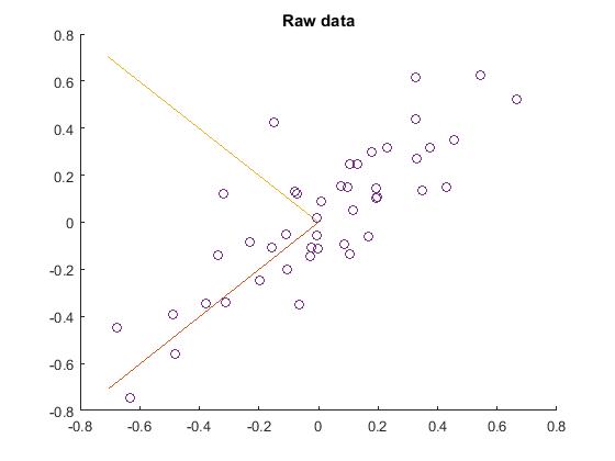
1.加载45个二维数据点,并用scatter函数显示出来。结果如下:

2.找到PCA的两个主方向,即:PCA的基,在原始数据上显示出来。先求出原始数据的协方差矩阵,再用svd函数求出该矩阵的特征向量,这就是要求的基。注意:对二维数据,其原始数据的预处理并没有0均值归一化。结果如下:
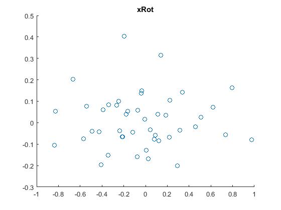
3.把原始数据映射(投影)或旋转到上一步所求的基方向上,得到数据 ,然后用scatter函数把它显示出来。结果如下:
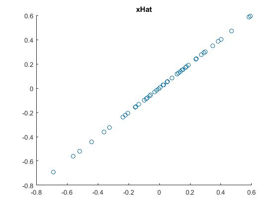
4.降维后近似还原原始数据,即:对上一步的数据结果降维,并显示出来。先计算设置要保留下来的主成份个数k,从而计算出降维后还原的原始数据  。结果如下:
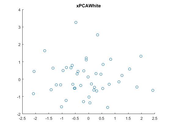
5.PCA白化,即把原始数据利用PCA whitening的方法去相关后,得到的原数据显示出来。结果如下:
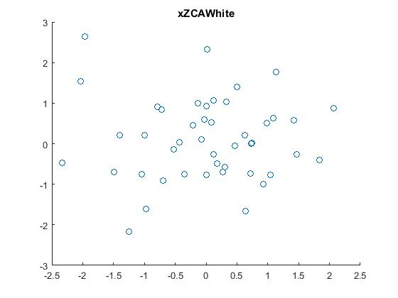
6.ZCA白化,即把原始数据利用ZCA whitening的方法去相关后,得到的原数据显示出来。结果如下:
代码
pca_2d.m
close all

%%================================================================
%% Step 0: Load data
%  We have provided the code to load data from pcaData.txt into x.
%  x is a 2 * 45 matrix, where the kth column x(:,k) corresponds to
%  the kth data point.Here we provide the code to load natural image data into x.
%  You do not need to change the code below.

x = load('pcaData.txt','-ascii');
figure(1);
scatter(x(1, :), x(2, :));
title('Raw data');


%%================================================================
%% Step 1a: Implement PCA to obtain U
%  Implement PCA to obtain the rotation matrix U, which is the eigenbasis
%  sigma.

% -------------------- YOUR CODE HERE --------------------
u = zeros(size(x, 1)); % You need to compute this
[n m] = size(x);
%x = x-repmat(mean(x,2),1,m);%预处理,均值为0
sigma = (1.0/m)*x*x';
[u s v] = svd(sigma);


% --------------------------------------------------------
hold on
plot([0 u(1,1)], [0 u(2,1)]);%画第一条线
plot([0 u(1,2)], [0 u(2,2)]);%第二条线
scatter(x(1, :), x(2, :));
hold off

%%================================================================
%% Step 1b: Compute xRot, the projection on to the eigenbasis
%  Now, compute xRot by projecting the data on to the basis defined
%  by U. Visualize the points by performing a scatter plot.

% -------------------- YOUR CODE HERE --------------------
xRot = zeros(size(x)); % You need to compute this
xRot = u'*x;


% --------------------------------------------------------

% Visualise the covariance matrix. You should see a line across the
% diagonal against a blue background.
figure(2);
scatter(xRot(1, :), xRot(2, :));
title('xRot');

%%================================================================
%% Step 2: Reduce the number of dimensions from 2 to 1.
%  Compute xRot again (this time projecting to 1 dimension).
%  Then, compute xHat by projecting the xRot back onto the original axes
%  to see the effect of dimension reduction

% -------------------- YOUR CODE HERE --------------------
k = 1; % Use k = 1 and project the data onto the first eigenbasis
xHat = zeros(size(x)); % You need to compute this
xHat = u*([u(:,1),zeros(n,1)]'*x);


% --------------------------------------------------------
figure(3);
scatter(xHat(1, :), xHat(2, :));
title('xHat');


%%================================================================
%% Step 3: PCA Whitening
%  Complute xPCAWhite and plot the results.

epsilon = 1e-5;
% -------------------- YOUR CODE HERE --------------------
xPCAWhite = zeros(size(x)); % You need to compute this
xPCAWhite = diag(1./sqrt(diag(s)+epsilon))*u'*x;


% --------------------------------------------------------
figure(4);
scatter(xPCAWhite(1, :), xPCAWhite(2, :));
title('xPCAWhite');

%%================================================================
%% Step 3: ZCA Whitening
%  Complute xZCAWhite and plot the results.

% -------------------- YOUR CODE HERE --------------------
xZCAWhite = zeros(size(x)); % You need to compute this
xZCAWhite = u*diag(1./sqrt(diag(s)+epsilon))*u'*x;

% --------------------------------------------------------
figure(5);
scatter(xZCAWhite(1, :), xZCAWhite(2, :));
title('xZCAWhite');

%% Congratulations! When you have reached this point, you are done!
%  You can now move onto the next PCA exercise. :)
二维数据:pcaData.txt
  -6.7644914e-01  -6.3089308e-01  -4.8915202e-01  -4.8005424e-01  -3.7842021e-01  -3.3788391e-01  -3.2023528e-01  -3.1108837e-01  -2.3145555e-01  -1.9623727e-01  -1.5678926e-01  -1.4900779e-01  -1.0861557e-01  -1.0506308e-01  -8.0899829e-02  -7.1157518e-02  -6.3251073e-02  -2.6007219e-02  -2.2553443e-02  -5.8489047e-03  -4.3935323e-03  -1.7309716e-03   7.8223728e-03   7.5386969e-02   8.6608396e-02   9.6406046e-02   1.0331683e-01   1.0531131e-01   1.1493296e-01   1.3052813e-01   1.6626253e-01   1.7901863e-01   1.9267343e-01   1.9414427e-01   1.9770003e-01   2.3043613e-01   3.2715844e-01   3.2737163e-01   3.2922364e-01   3.4869293e-01   3.7500704e-01   4.2830153e-01   4.5432503e-01   5.4422436e-01   6.6539963e-01
  -4.4722050e-01  -7.4778067e-01  -3.9074344e-01  -5.6036362e-01  -3.4291940e-01  -1.3832158e-01   1.2360939e-01  -3.3934986e-01  -8.2868433e-02  -2.4759514e-01  -1.0914760e-01   4.2243921e-01  -5.2329327e-02  -2.0126541e-01   1.3016657e-01   1.2293321e-01  -3.4787750e-01  -1.4584897e-01  -1.0559656e-01  -5.4200847e-02   1.6915422e-02  -1.1069762e-01   9.0859816e-02   1.5269096e-01  -9.4416463e-02   1.5116385e-01  -1.3540126e-01   2.4592698e-01   5.1087447e-02   2.4583340e-01  -5.9535372e-02   2.9704742e-01   1.0168115e-01   1.4258649e-01   1.0662592e-01   3.1698532e-01   6.1577841e-01   4.3911172e-01   2.7156501e-01   1.3572389e-01   3.1918066e-01   1.5122962e-01   3.4979047e-01   6.2316971e-01   5.2018811e-01
参考资料:
http://www.cnblogs.com/tornadomeet/archive/2013/03/21/2973631.html