ggplot2（7）定位

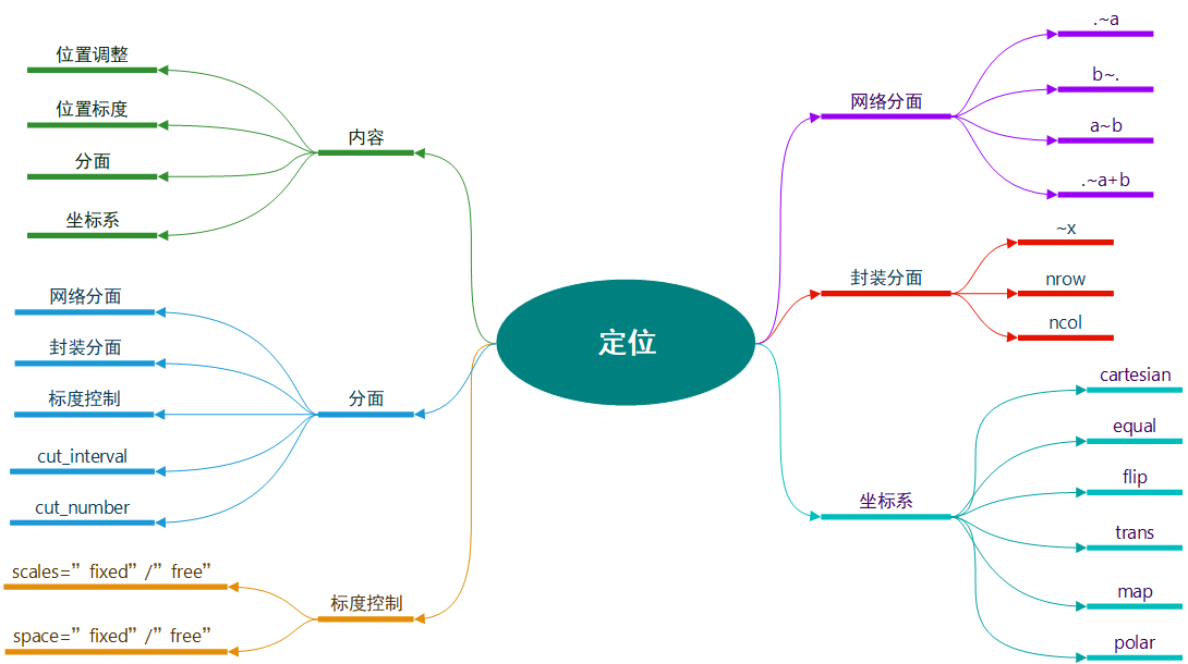
7.1 简介

位置调整：调整每个图层中出现重叠的对象的位置，对条形图和其他有组距的图形非常有用；
位置标度：控制数据到图形中位置的映射，常用的是对数变换；
分面：先将数据集划分为多个子集，然后将每个子集依次绘制到页面的不同面板中；
坐标系：通过控制两个独立的位置标度来生成一个2维的坐标系。

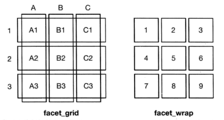
7.2 分面

facet_grid（网络型）：面板的行与列通过变量来定义（使用x~y定义）；
facet_wrap（封装型）：将1维面板封装到2维中（使用~x定义）。

分面绘图通常会占用大量空间。

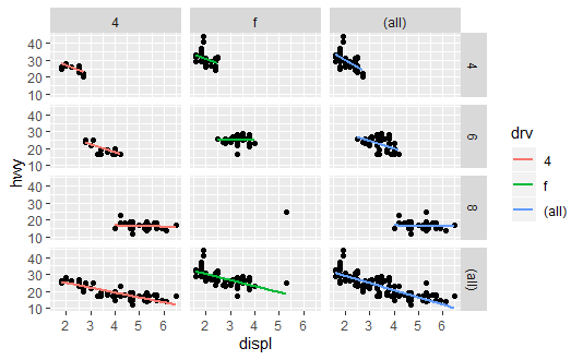
7.2.1 网络分面

一行多列（".~a"）：有助于y方向的比较；
多行一列（"b~."）：有助于x方向的比较，尤其是数据分布的比较；
多行多列（"a~b"）：通常行数小于列数，以充分利用屏幕；
多个变量在一行或列上（".~a+b"或"a+b~."）：使用较少。

边际图：使用margins = TRUE可以展示所有的边际图。

mpg2 <- subset(mpg, cyl != 5 & drv %in% c("4", "f"))

###### 章节7.2.1
p <- qplot(displ, hwy, data = mpg2) + 
  geom_smooth(aes(colour = drv),method = "lm", se = F)
p + facet_grid(cyl ~ drv, margins = T)

7.2.2 封装分面

例：

https://www.cnblogs.com/dingdangsunny/p/12327916.html#_label1_2

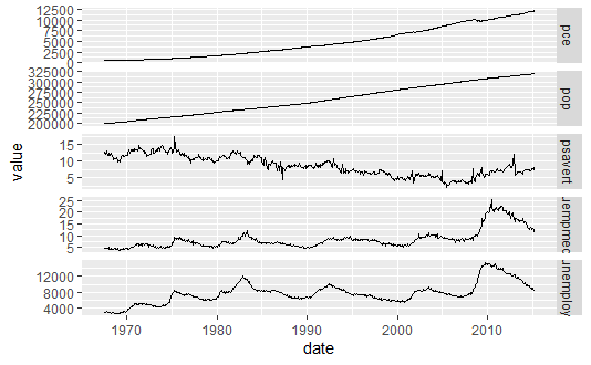
7.2.3 标度控制

scales = "fixed"：x和y的标度在所有面板中都相同；
scales = "free"：x和y的标度在每个面板中都可以变化；
scales = "free_x"：x标度可变，y尺度固定；
scales = "free_y"：y标度可变，x尺度固定。

同列的面板必须拥有相同的x标度，同行的面板必须拥有相同的y标度。

library(reshape2)
em <- melt(economics, id = "date")
# 0.9.0版本中 melt() 函数需要加载 reshape2 包
qplot(date, value, data = em, geom = "line", group = variable) + 
  facet_grid(variable ~ ., scale = "free_y")

space = "free"：每行（列）的高度（宽度）与该行（列）的标度范围成正比，这将使得所有面板的标度比例相同。
space = "fixed"：固定均分。

models <- qplot(displ, hwy, data = mpg)

models
models + facet_grid(drv ~ ., scales = "free", space = "free") + theme(strip.text.y = element_text())
models + facet_grid(drv ~ ., scales = "free", space = "fixed") + theme(strip.text.y = element_text())

7.2.4 分组与分面

分面相距较远，组间无重叠，在组与组之间可能会重叠时有优势；分组各组绘制在同一面板，容易发现组间细微的差别。

另外，分面在比较两个变量相对于两个不同的图形属性时更为容易，分面的另一优势是数据子集若有不同的尺度范围，各个面板可以做出相应调整。

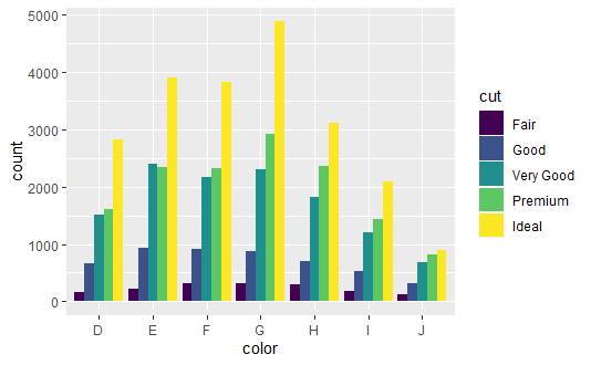
7.2.5 并列与分面

dplot <- ggplot(diamonds, aes(color, fill = cut))
dplot + geom_bar(position = "dodge")
qplot(cut, data = diamonds, geom = "bar", fill = cut) + facet_grid(. ~ color) + 
    theme(axis.text.x = element_text(angle = 90, hjust = 1, size = 8, colour = "grey50"))

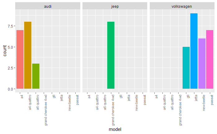
mpg4 <- subset(mpg, manufacturer %in% c("audi", "volkswagen", "jeep"))
mpg4$manufacturer <- as.character(mpg4$manufacturer)
mpg4$model <- as.character(mpg4$model)

base <- ggplot(mpg4, aes(fill = model)) + geom_bar(position = "dodge") + theme(legend.position = "none")

base + aes(x = model) + facet_grid(. ~ manufacturer) + 
    theme(axis.text.x = element_text(angle = 90, hjust = 1, size = 8, colour = "grey50"))
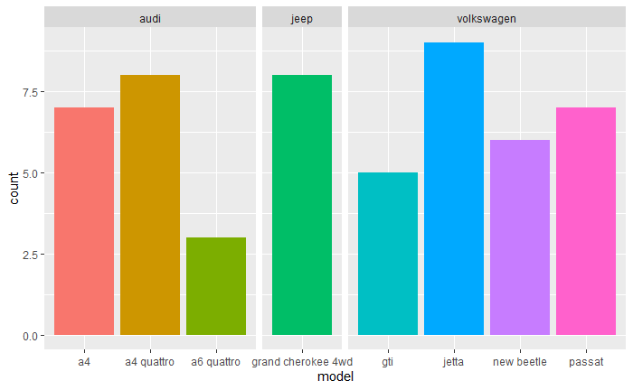
base + aes(x = model) + facet_grid(. ~ manufacturer) + 
  facet_grid(. ~ manufacturer, scales = "free_x", space = "free")
base + aes(x = manufacturer)

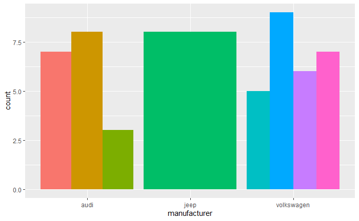
水平完全交叉：分面与并列基本相同；
水平几乎交叉：有相同标度的分面保证了所有的水平组合可见，即使有些是空的；
水平无交叉：标度自由的分面会对每个有较高水平的组别分配完全充足的作图空间，并对每个条目都进行标注。

7.2.6 连续型变量

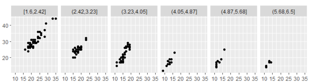
使用cut_interval(x, n = 10)将数据划分为n个长度相同的部分，n控制划分数目；
使用cut_interval(x,length = 1)将数据划分为若干个长度相同的部分，每个部分的长度为length；
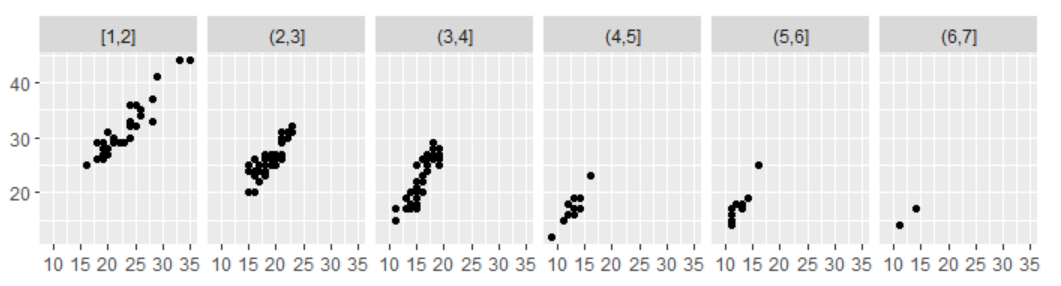
使用cut_number(x, n = 10)将数据划分为具有相同点数的部分，使得每个分面中有相同的点数，对比更容易，但是需要注意每个部分的标度范围是不同的。

mpg2$disp_ww <- cut_interval(mpg2$displ, length = 1)
mpg2$disp_wn <- cut_interval(mpg2$displ, n = 6)
mpg2$disp_nn <- cut_number(mpg2$displ, n = 6)

plot <- qplot(cty, hwy, data = mpg2) + labs(x = NULL, y = NULL)
plot + facet_wrap(~disp_ww, nrow = 1)
plot + facet_wrap(~disp_wn, nrow = 1)
plot + facet_wrap(~disp_nn, nrow = 1)

7.3 坐标系

坐标系是将两种位置标度结合在一起组成的2维定位系统。

名称	描述
cartesian	笛卡尔坐标系
equal	同尺度笛卡尔坐标系
flip	翻转的笛卡尔坐标系
trans	变换的笛卡尔坐标系
map	地图射影
polar	极坐标系

注：coord_equal和coord_fixed等价。

7.3.1 变换

坐标变换分为两步：首先，几何形状的参数变换只依据定位，而不是定位和维度；下一步就是将每个位置转化到新的坐标系中。

d<-data.frame(x = 1:100, y = 1:100)
qplot(x, y, data = d, geom = "line") + coord_equal()
qplot(x, y, data = d, geom = "line") + coord_polar()

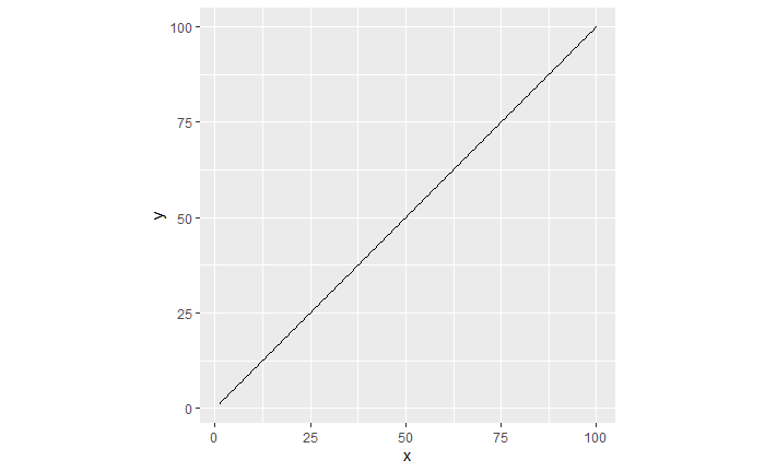
直角坐标系中的直线在极坐标系中变为螺线。

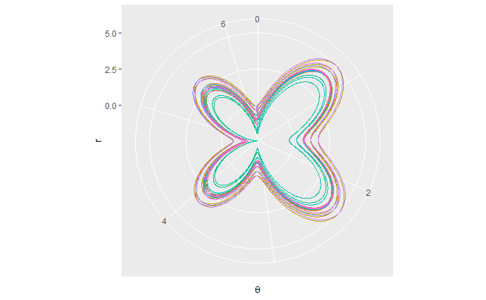
蝴蝶线：

th_x < -rep(seq(0, 2*pi, 0.005), 20)
th <- seq(0, 40*pi, 0.005)
r <- exp(sin(th)) - 2 * cos(4 * th) + (sin((2*th - pi) / 24))^5
th_n <- cut_number(th, n = 20)
qplot(th_x[1:length(th)], r, colour = th_n, geom = "line") + coord_polar() + 
  guides(colour = F) + labs(x=expression(theta))

7.3.2 笛卡尔坐标系

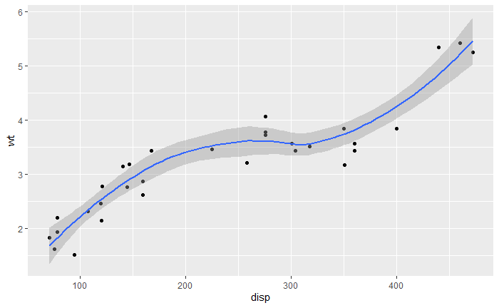
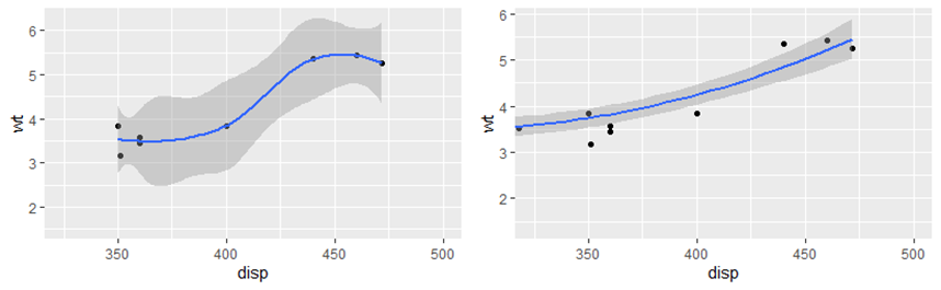
设置范围

coord_cartesian有xlim和ylim参数，局部放大图形。

(p <- qplot(disp, wt, data = mtcars) + geom_smooth())
p + scale_x_continuous(limits = c(325, 500))
p + coord_cartesian(xlim = c(325, 500))

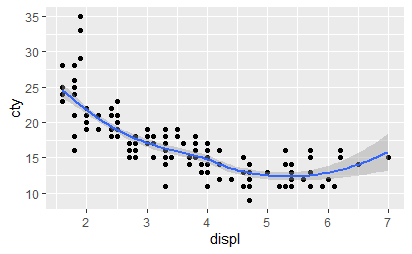
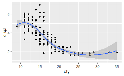
坐标轴翻转

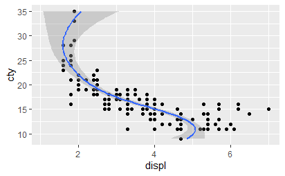
使用coord_flip调换x和y轴。

qplot(displ, cty, data = mpg) + geom_smooth()
qplot(cty, displ, data = mpg) + geom_smooth()
qplot(cty, displ, data = mpg) + geom_smooth() + 
  coord_flip()

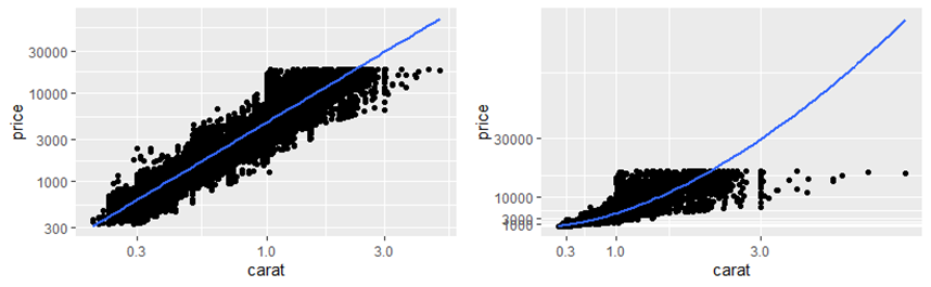
变换

qplot(carat, price, data = diamonds, log = "xy") + geom_smooth(method = "lm")
## 译者注: 原书中为'pow10'，0.9.0 中为 exp_trans(10)，且需加载scales包
library(scales)
last_plot() + coord_trans(x = exp_trans(10), y = exp_trans(10))

相同标度

coord_equal保证x轴和y轴有相同的标度。默认1：1，通过修改ratio可以进行修改。

coord_fixed(ratio = 1, xlim = NULL, ylim = NULL, expand = TRUE, clip = "on")

7.3.3 非笛卡尔坐标系

极坐标

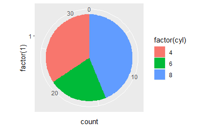
极坐标系统最常用于饼图，饼图是在极坐标下堆叠的条形图。

coord_polar(theta = "x", start = 0, direction = 1, clip = "on")

theta：将角度映射到(x或y)的变量；
start：起始点从12点的偏移量(以弧度表示)；
direction：1表示顺时针方，-1表示逆时针方向；

# A pie chart = stacked bar chart + polar coordinates
pie <- ggplot(mtcars, aes(x = factor(1), fill = factor(cyl))) +
 geom_bar(width = 1)
pie + coord_polar(theta = "y")

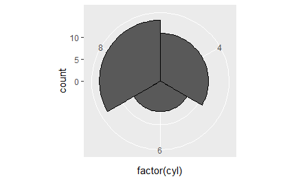
# A coxcomb plot = bar chart + polar coordinates
cxc <- ggplot(mtcars, aes(x = factor(cyl))) +
  geom_bar(width = 1, colour = "black")
cxc + coord_polar()

# The bullseye chart
pie + coord_polar()

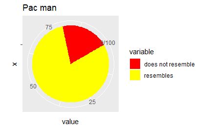
# Hadley's favourite pie chart
df <- data.frame(
  variable = c("does not resemble", "resembles"),
  value = c(20, 80)
)
ggplot(df, aes(x = "", y = value, fill = variable)) +
  geom_col(width = 1) +
  scale_fill_manual(values = c("red", "yellow")) +
  coord_polar("y", start = pi / 3) +
  labs(title = "Pac man")

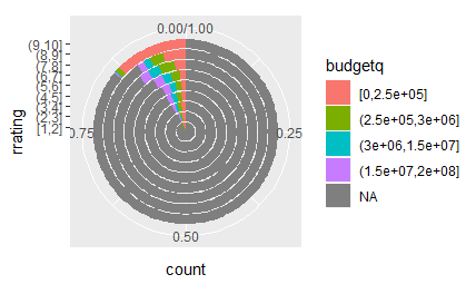
# Windrose + doughnut plot
if (require("ggplot2movies")) {
movies$rrating <- cut_interval(movies$rating, length = 1)
movies$budgetq <- cut_number(movies$budget, 4)

doh <- ggplot(movies, aes(x = rrating, fill = budgetq))

# Wind rose
doh + geom_bar(width = 1) + coord_polar()
# Race track plot
doh + geom_bar(width = 0.9, position = "fill") + coord_polar(theta = "y")
}

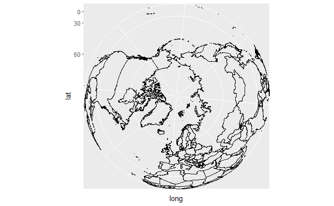
地图

世界地图：

if (require("maps")) {
# World map, using geom_path instead of geom_polygon
world <- map_data("world")
worldmap <- ggplot(world, aes(x = long, y = lat, group = group)) +
  geom_path() +
  scale_y_continuous(breaks = (-2:2) * 30) +
  scale_x_continuous(breaks = (-4:4) * 45)

# Orthographic projection with default orientation (looking down at North pole)
worldmap + coord_map("ortho")
}

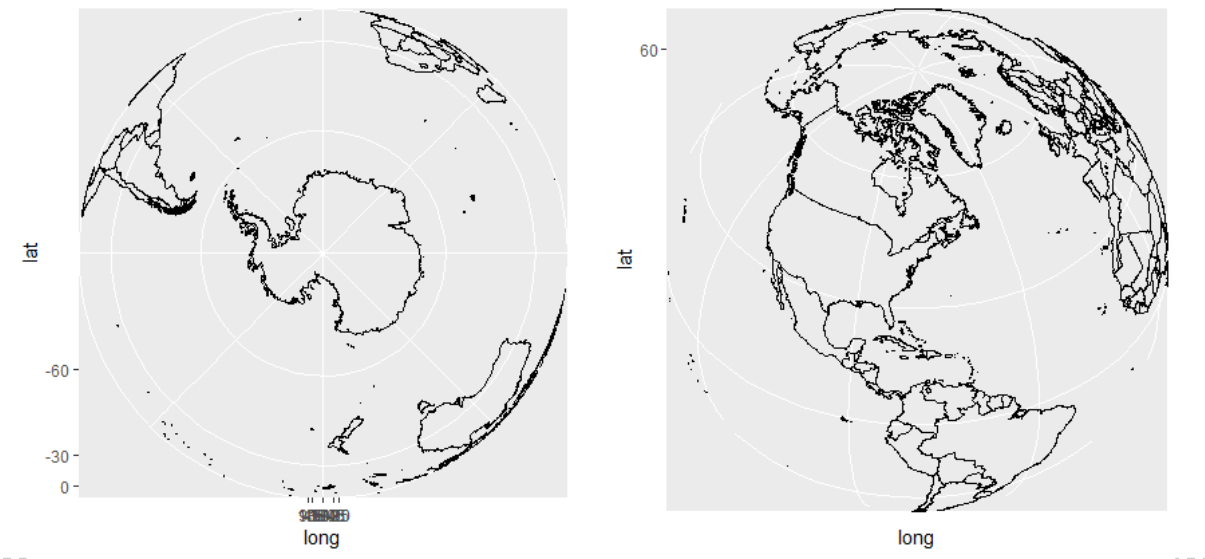
if (require("maps")) {
# Looking up up at South Pole
worldmap + coord_map("ortho", orientation = c(-90, 0, 0))
}

if (require("maps")) {
# Centered on New York (currently has issues with closing polygons)
worldmap + coord_map("ortho", orientation = c(41, -74, 0))
}

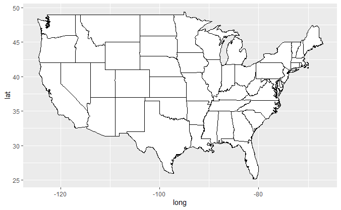
美国地图

if (require("maps")) {
states <- map_data("state")
usamap <- ggplot(states, aes(long, lat, group = group)) +
  geom_polygon(fill = "white", colour = "black")

# Use cartesian coordinates
usamap
}

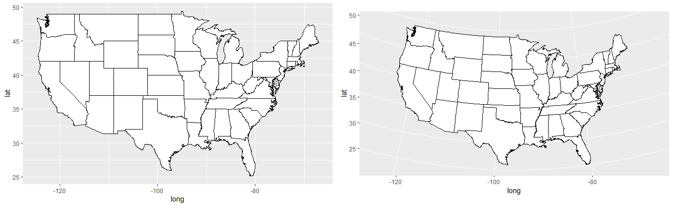
if (require("maps")) {
usamap + coord_map("conic", lat0 = 30)
}

if (require("maps")) {
usamap + coord_map("bonne", lat0 = 50)
}

其他示例在https://www.cnblogs.com/dingdangsunny/p/12354072.html#_label6

ggplot2（7） 定位