一.回归模型与房价预测
要求:
1. 导入boston房价数据集
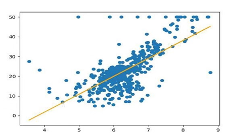
2. 一元线性回归模型,建立一个变量与房价之间的预测模型,并图形化显示。
3. 多元线性回归模型,建立13个变量与房价之间的预测模型,并检测模型好坏,并图形化显示检查结果。
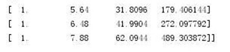
4. 一元多项式回归模型,建立一个变量与房价之间的预测模型,并图形化显示。
#导入波士顿房价数据集
from sklearn.datasets import load_boston
import  pandas as pd

boston = load_boston()
df = pd.DataFrame(boston.data)

#一元线性回归模型,建立一个变量与房价之间的预测模型,并图形化显示。
from sklearn.linear_model import LinearRegression
import  matplotlib.pyplot as plt

x =boston.data[:,5]
y = boston.target
LinR = LinearRegression()
LinR.fit(x.reshape(-1,1),y)
w=LinR.coef_
b=LinR.intercept_
print(w,b)

plt.scatter(x,y)
plt.plot(x,w*x+b,'orange')
plt.show()

#多元线性回归模型,建立13个变量与房价之间的预测模型,并检测模型好坏,并图形化显示检查结果。
x = boston.data[:,12].reshape(-1,1)
y = boston.target
plt.figure(figsize=(10,6))
plt.scatter(x,y)

lineR = LinearRegression()
lineR.fit(x,y)
y_pred = lineR.predict(x)
plt.plot(x,y_pred,'r')
print(lineR.coef_,lineR.intercept_)
plt.show()

#一元多项式回归模型,建立一个变量与房价之间的预测模型,并图形化显示。

from sklearn.preprocessing import PolynomialFeatures
poly = PolynomialFeatures(degree=3)
x_poly = poly.fit_transform(x)
print(x_poly)
lrp = LinearRegression()
lrp.fit(x_poly,y)
y_poly_pred = lrp.predict(x_poly)
plt.scatter(x,y)
plt.scatter(x,y_pred)
plt.scatter(x,y_poly_pred)
plt.show()

# 多元线性回归模型
from sklearn.datasets import load_boston
from sklearn.model_selection import train_test_split

# 波士顿房价数据集
data = load_boston()

# 划分数据集
x_train, x_test, y_train, y_test = train_test_split(data.data,data.target,test_size=0.3)

# 建立多元线性回归模型
mlr = LinearRegression()
mlr.fit(x_train,y_train)
print('系数',mlr.coef_,"
截距",mlr.intercept_)

# 检测模型好坏
from sklearn.metrics import regression
y_predict = mlr.predict(x_test)
# 计算模型的预测指标
print("预测的均方误差:", regression.mean_squared_error(y_test,y_predict))
print("预测的平均绝对误差:", regression.mean_absolute_error(y_test,y_predict))
# 打印模型的分数
print("模型的分数:",mlr.score(x_test, y_test))

# 多元多项式回归模型
# 多项式化
poly2 = PolynomialFeatures(degree=2)
x_poly_train = poly2.fit_transform(x_train)
x_poly_test = poly2.transform(x_test)

# 建立模型
mlrp = LinearRegression()
mlrp.fit(x_poly_train, y_train)

# 预测
y_predict2 = mlrp.predict(x_poly_test)

# 检测模型好坏
# 计算模型的预测指标
print("预测的均方误差:", regression.mean_squared_error(y_test,y_predict2))
print("预测的平均绝对误差:", regression.mean_absolute_error(y_test,y_predict2))
# 评估模型的分数
print("模型的分数:",mlrp.score(x_poly_test, y_test))
运行结果:
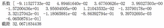
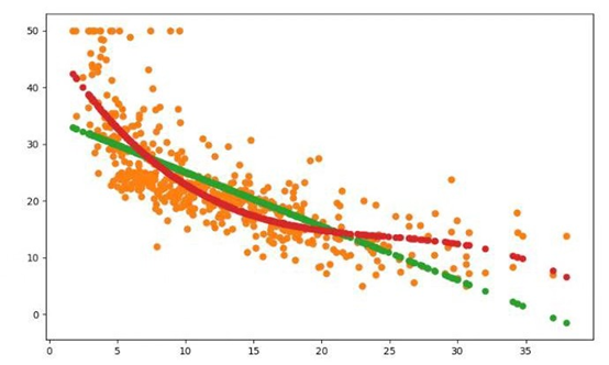
建立13个变量与房价之间多元回归模型
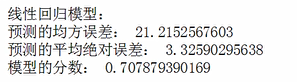
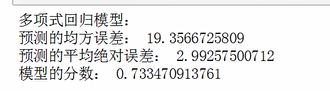
检测线性回归模型的好坏

结论:
通过比较一元线性回归模型和多元线性回归模型,会发现,多元线性回归模型所见的曲线比一元线性回归模型的直线更贴合样本点的分布。所以,多元线性回归模型更优,性能更好,误差更小。
二.中文文本分类
要求:
按学号末位下载相应数据集。
258:家居、教育、科技、社会、时尚、
分别建立中文文本分类模型,实现对文本的分类。
基本步骤如下:
1.各种获取文件,写文件
2.除去噪声,如:格式转换,去掉符号,整体规范化
3.遍历每个个文件夹下的每个文本文件。
4.使用jieba分词将中文文本切割。
中文分词就是将一句话拆分为各个词语,因为中文分词在不同的语境中歧义较大,所以分词极其重要。
可以用jieba.add_word('word')增加词,用jieba.load_userdict('wordDict.txt')导入词库。
维护自定义词库
5.去掉停用词。
维护停用词表
6.对处理之后的文本开始用TF-IDF算法进行单词权值的计算
7.贝叶斯预测种类
8.模型评价
9.新文本类别预测
处理过程中注意:
- 实验过程中文件遍历从少量到多量,调试无误后再处理全部文件
- 判断文件大小决定读取方法
- 注意保存中间结果,以免每次从头读取文件重复处理
- 内存不足时进行分批处理
- 利用数组的保存np.save('x1.npy',x1)与数组的读取np.load('x1.npy')和数组的拼接np.concatenate((x1,x2),axis=0)
- 及时用 del(x1) 释放大块内存,用gc.collect()回收内存。
- 边处理边保存数据,不要处理完了一次性保存。万一中间发生的异常情况,就全部白做了。
- 进行Python 异常处理,把出错的文件单独记录,程序可以继续执行。回头再单独处理出错的文件。
在准备长时间无监督运行程序之前,请关闭windows自动更新、自动屏保关机等...
代码:
# 导入数据
import os
import numpy as np
import sys
from datetime import datetime
import gc
path = 'C:\Users\s2009\Desktop\dididi\258'

# 导入结巴库
import jieba
# 加载停用词赋值给变量
with open(r'258stopsCN.txt', encoding='utf-8') as f:
stopwords = f.read().split('
')

#定义函数处理文本,字符串
def processing(tokens):
    # 去掉非字母汉字的字符
    tokens = "".join([char for char in tokens if char.isalpha()])
    # 结巴分词,保留长度大于2的词
    tokens = [token for token in jieba.cut(tokens,cut_all=True) if len(token) >=2]
    # 删除停用词
    tokens = " ".join([token for token in tokens if token not in stopwords])
return tokens

# 将处理好的数据放入文本列表和标签列表
tokenList = []
targetList = []
# 在os包下调用walk方法获取需要的变量,并返回文件根目录,文件夹名称,文件名,最后得到每个新闻的路径
for root,dirs,files in os.walk(path):
    for f in files:
        filePath = os.path.join(root,f)
        with open(filePath, encoding='utf-8') as f:
            content = f.read()
   # 获取新闻类别标签,并处理该新闻
        target = filePath.split('\')[-2]
        targetList.append(target)
        tokenList.append(processing(content))


#划分训练集,测试集,用TF-IDF算法计算单词权值
from sklearn.feature_extraction.text import TfidfVectorizer
from sklearn.model_selection import train_test_split
from sklearn.naive_bayes import GaussianNB,MultinomialNB
from sklearn.model_selection import cross_val_score
from sklearn.metrics import classification_report
x_train,x_test,y_train,y_test = train_test_split(tokenList,targetList,test_size=0.2,stratify=targetList)
# 数据向量化处理,选择TfidfVectorizer的方式建立特征向量。
vectorizer = TfidfVectorizer()
X_train = vectorizer.fit_transform(x_train)
X_test = vectorizer.transform(x_test)
# 建立模型,使用多项式朴素贝叶斯,调用fit方法
mnb = MultinomialNB()
module = mnb.fit(X_train, y_train)

#对模型进行预测
y_predict = module.predict(X_test)
# 输出模型精确度
scores=cross_val_score(mnb,X_test,y_test,cv=5)
print("Accuracy:%.3f"%scores.mean())
# 输出模型评估报告
print("classification_report:
",classification_report(y_predict,y_test))


# 将预测结果和实际结果进行对比
import collections
import matplotlib.pyplot as plt
from pylab import mpl
mpl.rcParams['font.sans-serif'] = ['FangSong'] # 指定默认字体
mpl.rcParams['axes.unicode_minus'] = False # 解决保存图像是负号'-'显示为方块的问题

# 统计测试集和预测集的各类新闻个数
testCount = collections.Counter(y_test)
predCount = collections.Counter(y_predict)
print('实际:',testCount,'
', '预测', predCount)


# 建立标签列表,实际结果列表,预测结果列表,
nameList = list(testCount.keys())
testList = list(testCount.values())
predictList = list(predCount.values())
x = list(range(len(nameList)))
print("新闻类别:",nameList,'
',"实际:",testList,'
',"预测:",predictList)
运行结果:
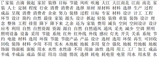
处理文本数据:去除停用词,保留长度大于2后得到的干净数据
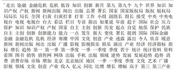
处理过的文本列表
查看标签列表,显示每个新闻的对应类别

建立的模型精确度为85.5%,下表显示精确度,召回度,f1值,支持度

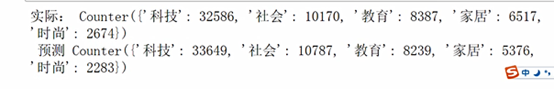
统计测试集和预测集的各类新闻个数
建立预测结果列表,实际结果列表
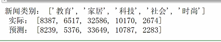
结论:检测后可知,此模型精确度较好,预测结果与实际结果差别不大