图 7.1


import matplotlib as mpl
import matplotlib.pyplot as plt
import numpy as np

mpl.rcParams["font.sans-serif"]=["SimHei"]
mpl.rcParams["axes.unicode_minus"]=False

fig, ax1 = plt.subplots()
t=np.arange(0.05, 10.0, 0.01)
s1=np.exp(t)
ax1.plot(t, s1, c="b", ls="-")

ax1.set_xlabel("x坐标轴")
ax1.set_ylabel("以e为底指数函数", color="b")
ax1.tick_params("y", colors="b")


ax2=ax1.twinx()

s2=np.cos(t**2)
ax2.plot(t, s2, c="r", ls=":")

ax2.set_ylabel("余弦函数", color="r")
ax2.tick_params("y", colors="r")

plt.show()
=====================================================
图 7.2
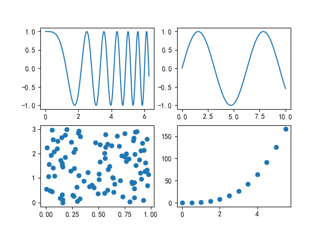
import matplotlib.pyplot as plt
import numpy as np

x1=np.linspace(0, 2*np.pi, 400)
y1=np.cos(x1**2)

x2=np.linspace(0.01, 10, 100)
y2=np.sin(x2)

x3=np.random.rand(100)
y3=np.linspace(0, 3, 100)

x4=np.arange(0, 6, 0.5)
y4=np.power(x4, 3)


fig, ax=plt.subplots(2, 2)


ax1=ax[0, 0]
ax1.plot(x1, y1)


ax2=ax[0, 1]
ax2.plot(x2, y2)


ax3=ax[1, 0]
ax3.scatter(x3, y3)


ax4=ax[1, 1]
ax4.scatter(x4, y4)


plt.show()
=====================================================
图 7.3

import matplotlib.pyplot as plt
import numpy as np

x1=np.linspace(0, 2*np.pi, 400)
y1=np.cos(x1**2)

x2=np.linspace(0.01, 10, 100)
y2=np.sin(x2)

x3=np.random.rand(100)
y3=np.linspace(0, 3, 100)

x4=np.arange(0, 6, 0.5)
y4=np.power(x4, 3)


fig, ax=plt.subplots(2, 2, sharex="all")


ax1=ax[0, 0]
ax1.plot(x1, y1)


ax2=ax[0, 1]
ax2.plot(x2, y2)


ax3=ax[1, 0]
ax3.scatter(x3, y3)


ax4=ax[1, 1]
ax4.scatter(x4, y4)


plt.show()
=====================================================
图 7.4
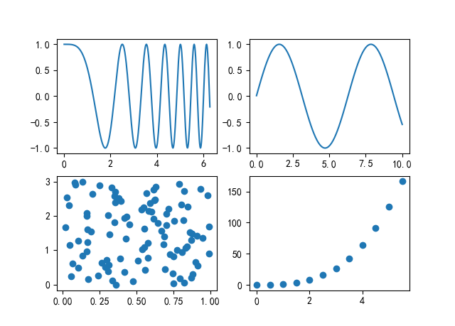
import matplotlib.pyplot as plt
import numpy as np

x1=np.linspace(0, 2*np.pi, 400)
y1=np.cos(x1**2)

x2=np.linspace(0.01, 10, 100)
y2=np.sin(x2)

x3=np.random.rand(100)
y3=np.linspace(0, 3, 100)

x4=np.arange(0, 6, 0.5)
y4=np.power(x4, 3)


fig, ax=plt.subplots(2, 2, sharex="none")


ax1=ax[0, 0]
ax1.plot(x1, y1)


ax2=ax[0, 1]
ax2.plot(x2, y2)


ax3=ax[1, 0]
ax3.scatter(x3, y3)


ax4=ax[1, 1]
ax4.scatter(x4, y4)


plt.show()
=====================================================
图 7.5
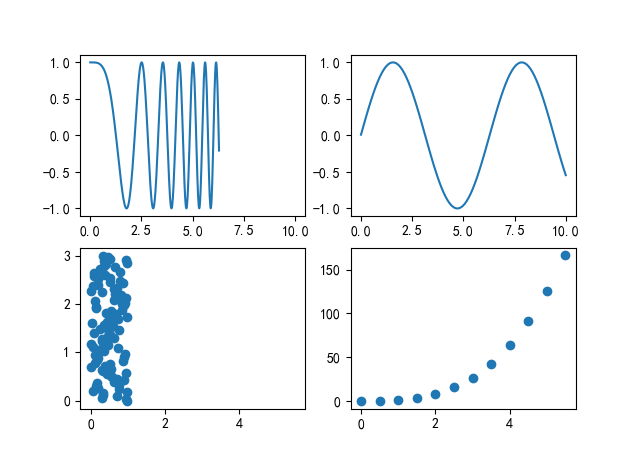
import matplotlib.pyplot as plt
import numpy as np

x1=np.linspace(0, 2*np.pi, 400)
y1=np.cos(x1**2)

x2=np.linspace(0.01, 10, 100)
y2=np.sin(x2)

x3=np.random.rand(100)
y3=np.linspace(0, 3, 100)

x4=np.arange(0, 6, 0.5)
y4=np.power(x4, 3)


fig, ax=plt.subplots(2, 2, sharex="row")


ax1=ax[0, 0]
ax1.plot(x1, y1)


ax2=ax[0, 1]
ax2.plot(x2, y2)


ax3=ax[1, 0]
ax3.scatter(x3, y3)


ax4=ax[1, 1]
ax4.scatter(x4, y4)


plt.show()
=====================================================
图 7.6
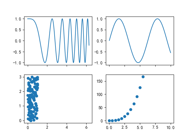
import matplotlib.pyplot as plt
import numpy as np

x1=np.linspace(0, 2*np.pi, 400)
y1=np.cos(x1**2)

x2=np.linspace(0.01, 10, 100)
y2=np.sin(x2)

x3=np.random.rand(100)
y3=np.linspace(0, 3, 100)

x4=np.arange(0, 6, 0.5)
y4=np.power(x4, 3)


fig, ax=plt.subplots(2, 2, sharex="col")


ax1=ax[0, 0]
ax1.plot(x1, y1)


ax2=ax[0, 1]
ax2.plot(x2, y2)


ax3=ax[1, 0]
ax3.scatter(x3, y3)


ax4=ax[1, 1]
ax4.scatter(x4, y4)


plt.show()
=====================================================
图 7.7
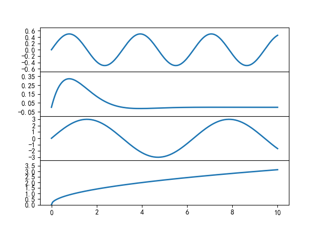
import matplotlib.pyplot as plt
import numpy as np

x=np.linspace(0.0, 10.0, 200)
y=np.cos(x)*np.sin(x)
y2=np.exp(-x)*np.sin(x)
y3=3*np.sin(x)
y4=np.power(x, 0.5)

fig, (ax1, ax2, ax3, ax4)=plt.subplots(4, 1, sharex="all")

fig.subplots_adjust(hspace=0)


ax1.plot(x, y, ls="-", lw=2)
ax1.set_yticks(np.arange(-0.6, 0.7, 0.2))
ax1.set_ylim(-0.7, 0.7)

ax2.plot(x, y2, ls="-", lw=2)
ax2.set_yticks(np.arange(-0.05, 0.36, 0.1))
ax2.set_ylim(-0.1, 0.4)

ax3.plot(x, y3, ls="-", lw=2)
ax3.set_yticks(np.arange(-3, 4, 1))
ax3.set_ylim(-3.5, 3.5)

ax4.plot(x, y4, ls="-", lw=2)
ax4.set_yticks(np.arange(0.0, 3.6, 0.5))
ax4.set_ylim(0.0, 4.0)

plt.show()
=====================================================
图 7.8

import matplotlib.pyplot as plt
import numpy as np

x1=np.linspace(0, 2*np.pi, 400)
y1=np.cos(x1**2)


x2=np.linspace(0.01, 10, 100)
y2=np.sin(x2)


x3=np.random.rand(100)
y3=np.linspace(0, 3, 100)


x4=np.arange(0, 6, 0.5)
y4=np.power(x4, 3)

fig, ax=plt.subplots(2, 2)

ax1=plt.subplot(221)
ax1.plot(x1, y1)

ax2=plt.subplot(222)
ax2.plot(x2, y2)


ax3=plt.subplot(223)
ax3.scatter(x3, y3)

ax4=plt.subplot(224, sharex=ax1)
ax4.scatter(x4, y4)


plt.show()
=====================================================
图 7.9

import matplotlib.pyplot as plt
import numpy as np

x1=np.linspace(0, 2*np.pi, 400)
y1=np.cos(x1**2)


x2=np.linspace(0.01, 10, 100)
y2=np.sin(x2)


x3=np.random.rand(100)
y3=np.linspace(0, 3, 100)


x4=np.arange(0, 6, 0.5)
y4=np.power(x4, 3)

fig, ax=plt.subplots(2, 2)

ax1=plt.subplot(221)
ax1.plot(x1, y1)

ax2=plt.subplot(222)
ax2.plot(x2, y2)


ax3=plt.subplot(223)

plt.autoscale(enable=True, axis="both", tight=True)

ax3.scatter(x3, y3)


ax4=plt.subplot(224, sharex=ax1)
ax4.scatter(x4, y4)


plt.show()
=====================================================