科学计算和可视化

一、Numpy

NumPy（Numeric Python）系统是 Python 的一种开源的数值计算扩展。这种工具可用来存储和处理大型矩阵，比 Python 自身的嵌套列表（nested list structure)结构要高效的多（该结构也可以用来表示矩阵（matrix））。据说 NumPy 将 Python 相当于变成一种免费的更强大的 MatLab 系统。

numpy 特性:开源，数据计算扩展，ndarray, 具有多维操作, 数矩阵数据类型、矢量处理，以及精密的运算库。专为进行严格的数字处理而产生。

特点：运算速度快、消耗资源少。

默认使用 Anaconda 集成包环境开发。

1、numpy 属性

几种 numpy 的属性：

ndim：维度
shape：行数和列数
size：元素个数

使用 numpy 首先要导入模块

1 import numpy as np #为了方便使用numpy 采用np简写

列表转化为矩阵：

array = np.array([[1,2,3],[2,3,4]])  #列表转化为矩阵
print(array)
"""
array([[1, 2, 3],
      [2, 3, 4]])
"""

numpy 的几种属性:

print('number of dim:',array.ndim)  # 维度
# number of dim: 2

print('shape :',array.shape)    # 行数和列数
# shape : (2, 3)

print('size:',array.size)   # 元素个数
# size: 6

2、Numpy 的创建 array

关键字

array：创建数组
dtype：指定数据类型
zeros：创建数据全为0
ones：创建数据全为1
empty：创建数据接近0
arrange：按指定范围创建数据
linspace：创建线段

二、Matplotlib

Matplotlib 是 Python 的绘图库。它可与 NumPy 一起使用，提供了一种有效的 MatLab 开源替代方案。它也可以和图形工具包一起使用，如 PyQt 和 wxPython。

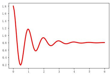
matplotlib.pyplot 模块可以画折线图，分为两个步骤，分别是 pyplot.plot() 和 pyplot.show() ，前者负责画图，后者将画好的图展示出来。

基本使用：

import numpy as np
import matplotlib.pyplot as plt
x=np.linspace(0,6,100)
y=np.cos(2*np.pi*x)*np.exp(-x)+0.8
plt.plot(x,y,'k',color='r',linewidth=3,linestyle="-")
plt.show()

效果如图：

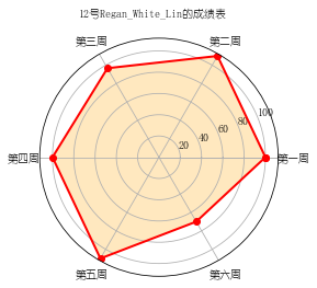
三、雷达图绘制

代码如下：

import numpy as np
import matplotlib.pyplot as plt
import matplotlib
matplotlib.rcParams['font.family']='YouYuan'
matplotlib.rcParams['font.sans-serif']=['YouYuan']
labels=np.array(['第一周','第二周','第三周','第四周','第五周','第六周'])
nAttr=6
data=np.array([100,100,96.7,100,110,70])
angles=np.linspace(0,2*np.pi,nAttr,endpoint=False)
data=np.concatenate((data,[data[0]]))
angles=np.concatenate((angles,[angles[0]]))
fig=plt.figure(facecolor="white")
plt.subplot(111,polar=True)
plt.plot(angles,data,'bo-',color='red',linewidth=2)
plt.fill(angles,data,facecolor='orange',alpha=0.25)
plt.thetagrids(angles*180/np.pi,labels)
plt.figtext(0.5,0.95,'12号Regan_White_Lin的成绩表',ha='center')
plt.grid(True)
plt.savefig('pic.JPG')
plt.show()

效果图如下：

四.散点图绘画

# -*- coding: utf-8 -*-
import numpy as np
import matplotlib.pyplot as plt

if __name__ == '__main__':
    print ("--------------散点图--------------")
    x = np.arange(50)
    print ("x")
    y = x + 5* np.random.rand(50)
    plt.scatter(x, y)
    plt.show()

运行结果：

五.自定义手绘风

from PIL import Image
import numpy as np

#为了便于文件的导入，可以使用相对路径，将文件和程序放在同一个文件夹下

vec_el=np.pi/2.2
vec_az=np.pi/4.
depth=10.
im=Image.open("HIT2.jpg").convert('L')
a=np.asarray(im).astype('float')
grad=np.gradient(a)
grad_x,grad_y=grad
grad_x=grad_x*depth/100.
grad_y=grad_y*depth/100.
dx=np.cos(vec_el)*np.cos(vec_az)
dy=np.cos(vec_el)*np.sin(vec_az)
dz=np.sin(vec_el)
A=np.sqrt(grad_x**2+grad_y**2+1.)
uni_x=grad_x/A
uni_y=grad_y/A
uni_z=1./A
a2=255*(dx*uni_x+dy*uni_y+dz*uni_z)
a2=a2.clip(0,255)
im2=Image.fromarray(a2.astype('uint8'))
im2.save('hit2-SH.jpg')
ils/82344288

原图：

手绘效果图：