sklearn.metrics中的confusion_matrix、ROC、AUC指标

1.confusion_matrix

理论部分见https://www.cnblogs.com/cxq1126/p/12990784.html#_label2

 1 from sklearn.metrics import confusion_matrix
 2 
 3 #if y_true.shape=y_pred.shape=(N,)
 4 tn, fp, fn, tp = confusion_matrix(y_true, y_pred, labels=[0, 1]).ravel()   
 5 print('sensitivity: ', tp/(tp+fn))
 6 print('specificity: ', tn/(tn+fp))
 7 
 8 #if y_true.shape=y_pred.shape=(N, 2)
 9 tn, fp, fn, tp = confusion_matrix(y_true2[:, 0], y_pred2[:, 0], labels=[0,1]).ravel()
10 print('sensitivity: ', tp/(tp+fn))
11 print('specificity: ', tn/(tn+fp))

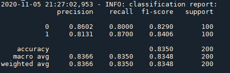
2.classification_report

1 from sklearn.metrics import classification_report
2 
3 file_logger.info('classification report:
%s' % classification_report(y_true, y_pred, target_names=test_dataset.ind_to_cls_dict, digits=4))

y_true和y_pred的shape=(N,)，结果类似下面

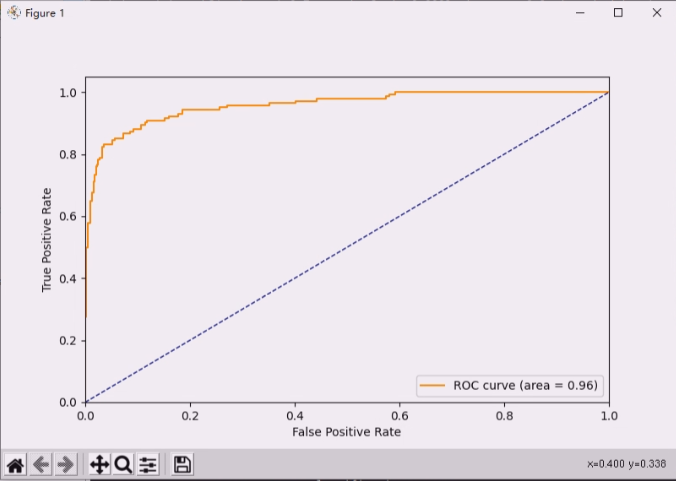
3.roc_curve, auc

如果最后的y_score维度是(N, )（即经过网络层的输出概率logits的shape=(N, )，也就是说最后的fc层输出维度为1），画一个ROC曲线

 1 from sklearn.metrics import roc_curve, auc 
 2 
 3 fpr, tpr, threshold = roc_curve(y_true, y_score)
 4 roc_auc = auc(fpr, tpr)
 5         
 6 plt.figure(figsize=(8, 5))
 7 plt.plot(fpr, tpr, color='darkorange', label='ROC curve (area = %0.4f)' % roc_auc)  
 8  
 9 lw = 2   
10 plt.plot([0, 1], [0, 1], color='navy', lw=lw, linestyle='--')
11 plt.xlim([0.0, 1.0])
12 plt.ylim([0.0, 1.05])
13 plt.xlabel('False Positive Rate')
14 plt.ylabel('True Positive Rate')
15 plt.legend(loc="lower right")
16 plt.show()

Tip：y_pred的类型是np.array

如果最后的y_score维度是(N, 2)（即经过网络层的输出概率logits的shape=(N, 2)，也就是说最后的fc层输出维度为2），按类别画2个ROC曲线

 1 from sklearn.metrics import roc_curve, auc 
 2 import matplotlib.pyplot as plt
 3 
 4 plt.figure(figsize=(8, 5))
 5 colors = ['darkorange', 'cornflowerblue']
 6 fpr, tpr, roc_auc = dict(), dict(), dict()
 7 for i in range(2):
 8      fpr[i], tpr[i], threshold = roc_curve(y_true2[:, i], y_score[:, i])
 9      roc_auc[i] = auc(fpr[i], tpr[i])
10         
11     
12      plt.plot(fpr[i], tpr[i], color=colors[i], label='ROC curve (area = %0.4f)' % roc_auc[i])  
13  
14 lw = 2   
15 plt.plot([0, 1], [0, 1], color='navy', lw=lw, linestyle='--')
16 plt.xlim([0.0, 1.0])
17 plt.ylim([0.0, 1.05])
18 plt.xlabel('1-Specificity')
19 plt.ylabel('Sensitivity')
20 plt.legend(loc="lower right")
21 plt.show()

如果维度(N,)想要转换成(N, 2)，可以使用独热编码，详细见https://www.cnblogs.com/cxq1126/p/13696082.html#_label3

1 import torch.nn.functional as F
2 
3 #y_true改成二维版本
4 x1 = F.one_hot(torch.tensor(y_true), num_classes = 2)
5 y_true2 = np.array(x1)

然后再调用roc_curve函数。