提前安装ffmpeg,参考https://www.cnblogs.com/Neeo/articles/11677715.html
1.逻辑回归解决二分类问题
1.1生成数据集
 1 import tensorflow as tf
 2 import matplotlib.pyplot as plt
 3
 4 from matplotlib import animation, rc
 5 from IPython.display import HTML
 6 import matplotlib.cm as cm
 7 import numpy as np
 8
 9
10 dot_num = 100
11 x_p = np.random.normal(3., 1, dot_num)
12 y_p = np.random.normal(6., 1, dot_num)
13 y = np.ones(dot_num)                                      #Y标签为1
14 C1 = np.array([x_p, y_p, y]).T
15
16 x_n = np.random.normal(6., 1, dot_num)
17 y_n = np.random.normal(3., 1, dot_num)
18 y = np.zeros(dot_num)                                     #Y标签为0
19 C2 = np.array([x_n, y_n, y]).T
20
21 plt.scatter(C1[:, 0], C1[:, 1], c='b', marker='+')        #高斯分布采样(X, Y) ~ N(3, 6, 1, 1, 0).
22 plt.scatter(C2[:, 0], C2[:, 1], c='g', marker='o')        #高斯分布采样 (X, Y) ~ N(6, 3, 1, 1, 0).
23
24 data_set = np.concatenate((C1, C2), axis=0)
25 np.random.shuffle(data_set)

1.2建立模型
逻辑函数的交叉熵损失函数: $=-sum _{i=1}^{n}y_ilog(p_i)+(1-y_i)log(1-p_i)$ $y_i$指i的真实值,$p_i$指i的预测值。
下面loss函数中在预测值pred后面加上了epsilon。
 1 epsilon = 1e-12
 2 class LogisticRegression():
 3     def __init__(self):
 4         self.W = tf.Variable(shape=[2, 1], dtype=tf.float32,
 5             initial_value=tf.random.uniform(shape=[2, 1], minval=-0.1, maxval=0.1))
 6         self.b = tf.Variable(shape=[1], dtype=tf.float32, initial_value=tf.zeros(shape=[1]))
 7
 8         self.trainable_variables = [self.W, self.b]
 9
10     @tf.function
11     def __call__(self, inp):
12         logits = tf.matmul(inp, self.W) + self.b         #shape(N, 1)
13         pred = tf.nn.sigmoid(logits)
14         return pred
15
16 @tf.function
17 def compute_loss(pred, label):
18     if not isinstance(label, tf.Tensor):
19         label = tf.constant(label, dtype=tf.float32)
20     pred = tf.squeeze(pred, axis=1)
21
22     '''============================='''
23     #输入label shape(N,), pred shape(N,)
24     #输出 losses shape(N,) 每一个样本一个loss
25     #todo 填空一,实现sigmoid的交叉熵损失函数(不使用tf内置的loss 函数)
26
27     #losses = -label*tf.math.log(pred) - (1-label)* tf.math.log(1-pred)
28     losses = -label*tf.math.log(pred+epsilon) - (1.-label)* tf.math.log(1.-pred+epsilon)
29      '''============================='''
30
31     loss = tf.reduce_mean(losses)
32
33     pred = tf.where(pred>0.5, tf.ones_like(pred), tf.zeros_like(pred))            #大于0.5预测正确,否则预测错误,形成判定矩阵
34     accuracy = tf.reduce_mean(tf.cast(tf.equal(label, pred), dtype=tf.float32))   #计算正确率
35     return loss, accuracy
36
37
38 @tf.function
39 def train_one_step(model, optimizer, x, y):
40     with tf.GradientTape() as tape:
41         pred = model(x)
42         loss, accuracy = compute_loss(pred, y)
43
44     grads = tape.gradient(loss, model.trainable_variables)
45     optimizer.apply_gradients(zip(grads, model.trainable_variables))
46     return loss, accuracy, model.W, model.b
1.3实例化一个模型,进行训练
 1 if __name__ == '__main__':
 2     model = LogisticRegression()
 3     opt = tf.keras.optimizers.SGD(learning_rate=0.01)              #SGD优化器
 4     x1, x2, y = list(zip(*data_set))
 5     x = list(zip(x1, x2))
 6     animation_fram = []
 7
 8     for i in range(200):
 9         loss, accuracy, W_opt, b_opt = train_one_step(model, opt, x, y)
10         animation_fram.append((W_opt.numpy()[0, 0], W_opt.numpy()[1, 0], b_opt.numpy(), loss.numpy()))
11         if i%20 == 0:
12             print(f'loss: {loss.numpy():.4}	 accuracy: {accuracy.numpy():.4}')
1.4展示动态结果
 1 f, ax = plt.subplots(figsize=(6,4))                             #f是图像对象,ax是坐标轴对象
 2 f.suptitle('Logistic Regression Example', fontsize=15)
 3 plt.ylabel('Y')
 4 plt.xlabel('X')
 5 ax.set_xlim(0, 10)
 6 ax.set_ylim(0, 10)
 7
 8 line_d, = ax.plot([], [], label='fit_line')
 9 C1_dots, = ax.plot([], [], '+', c='b', label='actual_dots')
10 C2_dots, = ax.plot([], [], 'o', c='g' ,label='actual_dots')
11
12
13 frame_text = ax.text(0.02, 0.95,'',horizontalalignment='left',verticalalignment='top', transform=ax.transAxes)
14
15 def init():
16     line_d.set_data([],[])
17     C1_dots.set_data([],[])
18     C2_dots.set_data([],[])
19     return (line_d,) + (C1_dots,) + (C2_dots,)
20
21 def animate(i):
22     xx = np.arange(10, step=0.1)
23     a = animation_fram[i][0]
24     b = animation_fram[i][1]
25     c = animation_fram[i][2]
26     yy = a/-b * xx +c/-b
27     line_d.set_data(xx, yy)
28
29     C1_dots.set_data(C1[:, 0], C1[:, 1])
30     C2_dots.set_data(C2[:, 0], C2[:, 1])
31
32     frame_text.set_text('Timestep = %.1d/%.1d
Loss = %.3f' % (i, len(animation_fram), animation_fram[i][3]))
33
34     return (line_d,) + (C1_dots,) + (C2_dots,)
35
36
37 #FuncAnimation函数绘制动图,f是画布,animate是自定义动画函数,init_func自定义开始帧,即传入init初始化函数,
38 #frames动画长度,一次循环包含的帧数,在函数运行时,其值会传递给函数animate(i)的形参“i”,interval更新频率,以ms计,blit选择更新所有点,还是仅更新产生变化的点。
39 anim = animation.FuncAnimation(f, animate, init_func=init, frames=len(animation_fram), interval=30, blit=True)
40 HTML(anim.to_html5_video())
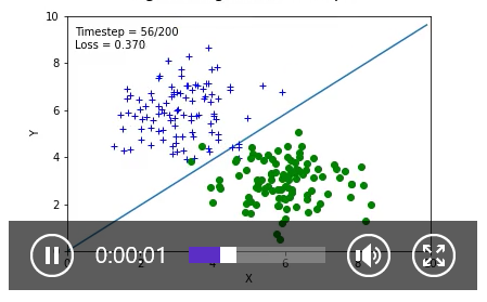
动态截图:
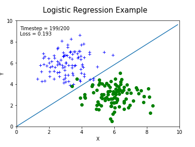
最终结果:
2.softmax回归解决多分类问题
2.1生成数据集
 1 import tensorflow as tf
 2 import matplotlib.pyplot as plt
 3
 4 from matplotlib import animation, rc
 5 from IPython.display import HTML
 6 import matplotlib.cm as cm
 7 import numpy as np
 8
 9
10 dot_num = 100
11 x_p = np.random.normal(3., 1, dot_num)
12 y_p = np.random.normal(6., 1, dot_num)
13 y = np.ones(dot_num)                                #Y标签为1
14 C1 = np.array([x_p, y_p, y]).T
15
16 x_n = np.random.normal(6., 1, dot_num)
17 y_n = np.random.normal(3., 1, dot_num)
18 y = np.zeros(dot_num)                               #Y标签为0
19 C2 = np.array([x_n, y_n, y]).T
20
21 x_b = np.random.normal(7., 1, dot_num)
22 y_b = np.random.normal(7., 1, dot_num)
23 y = np.ones(dot_num)*2                              #Y标签为2
24 C3 = np.array([x_b, y_b, y]).T
25
26 plt.scatter(C1[:, 0], C1[:, 1], c='b', marker='+')
27 plt.scatter(C2[:, 0], C2[:, 1], c='g', marker='o')
28 plt.scatter(C3[:, 0], C3[:, 1], c='r', marker='*')
29
30 data_set = np.concatenate((C1, C2, C3), axis=0)
31 np.random.shuffle(data_set)

2.2建立模型
softmax的交叉熵损失函数:$-frac{1}{N}sum _{n=1}^{N}sum _{c=1}^{C}y_{c}^{(n)}logp_{c}^{n}=-frac{1}{N}sum _{n=1}^{N}(y^{n})^{T}logp^{n}$ $y$指真实值,$p$指预测值。
下面loss函数中在预测值pred后面加上了epsilon。
 1 epsilon = 1e-12
 2 #建立模型类
 3 class SoftmaxRegression():
 4     def __init__(self):
 5         '''============================='''
 6         #todo 填空一,构建模型所需的参数 self.W, self.b 可以参考logistic-regression-exercise
 7         self.W = tf.Variable(shape=[2, 3], dtype=tf.float32, initial_value=tf.random.uniform(shape=[2, 3], minval=-0.1, maxval=0.1))
 8         self.b = tf.Variable(shape=[1, 3], dtype=tf.float32, initial_value=tf.zeros(shape=[1, 3]))
 9         '''============================='''
10
11         self.trainable_variables = [self.W, self.b]
12     @tf.function
13     def __call__(self, inp):
14         logits = tf.matmul(inp, self.W) + self.b             #shape(N, 3)
15         pred = tf.nn.softmax(logits)
16         return pred
17
18 #定义loss函数
19 @tf.function
20 def compute_loss(pred, label):
21     label = tf.one_hot(tf.cast(label, dtype=tf.int32), dtype=tf.float32, depth=3)
22     '''============================='''
23     #输入label shape(N, 3), pred shape(N, 3)
24     #输出 losses shape(N,) 每一个样本一个loss
25     #todo 填空二,实现softmax的交叉熵损失函数(不使用tf内置的loss 函数)
26     losses=-tf.reduce_mean(label*tf.math.log(pred+epsilon))
27     '''============================='''
28     loss = tf.reduce_mean(losses)
29
30     accuracy = tf.reduce_mean(tf.cast(tf.equal(tf.argmax(label,axis=1), tf.argmax(pred, axis=1)), dtype=tf.float32))
31     return loss, accuracy
32
33 #定义一步梯度下降过程函数
34 @tf.function
35 def train_one_step(model, optimizer, x, y):
36     with tf.GradientTape() as tape:
37         pred = model(x)
38         loss, accuracy = compute_loss(pred, y)
39
40     grads = tape.gradient(loss, model.trainable_variables)
41     optimizer.apply_gradients(zip(grads, model.trainable_variables))
42     return loss, accuracy
43
44
45 model = SoftmaxRegression()
46 opt = tf.keras.optimizers.SGD(learning_rate=0.01)
47 x1, x2, y = list(zip(*data_set))
48 x = list(zip(x1, x2))
49 for i in range(1000):
50     loss, accuracy = train_one_step(model, opt, x, y)
51     if i%50==49:
52         print(f'loss: {loss.numpy():.4}	 accuracy: {accuracy.numpy():.4}')
loss: 0.3311 accuracy: 0.36
loss: 0.2889 accuracy: 0.6433
loss: 0.2595 accuracy: 0.81
loss: 0.238 accuracy: 0.8667
loss: 0.2216 accuracy: 0.8767
loss: 0.2085 accuracy: 0.89
loss: 0.1979 accuracy: 0.8967
loss: 0.1889 accuracy: 0.9
loss: 0.1814 accuracy: 0.9033
loss: 0.1748 accuracy: 0.9067
loss: 0.1691 accuracy: 0.9067
loss: 0.164 accuracy: 0.9067
loss: 0.1595 accuracy: 0.9067
loss: 0.1554 accuracy: 0.9067
loss: 0.1517 accuracy: 0.9067
loss: 0.1484 accuracy: 0.9067
loss: 0.1453 accuracy: 0.9067
loss: 0.1425 accuracy: 0.9067
loss: 0.1398 accuracy: 0.9067
loss: 0.1374 accuracy: 0.9067
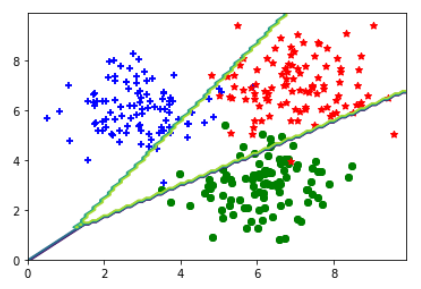
2.3展示结果
 1 plt.scatter(C1[:, 0], C1[:, 1], c='b', marker='+')
 2 plt.scatter(C2[:, 0], C2[:, 1], c='g', marker='o')
 3 plt.scatter(C3[:, 0], C3[:, 1], c='r', marker='*')
 4
 5 x = np.arange(0., 10., 0.1)
 6 y = np.arange(0., 10., 0.1)
 7
 8 X, Y = np.meshgrid(x, y)                          #生成网格点坐标矩阵(可形成100*100=10000个点坐标)
 9
10 inp = np.array(list(zip(X.reshape(-1), Y.reshape(-1))), dtype=np.float32)
11 print(inp.shape)                                  #(10000, 2),inp相当于10000个点坐标
12
13 Z = model(inp)                                    #Z.shape=(10000,3)
14 Z = np.argmax(Z, axis=1)                          #(10000,)选出三个类别中的最可能类别
15 Z = Z.reshape(X.shape)                            #(100,100)
16 plt.contour(X,Y,Z)                                #绘制等高线,Z看成关于X,Y的函数
17 plt.show()