machine learning Naive_Bayes_classifier (FINISHED)

http://en.wikipedia.org/wiki/Naive_Bayes_classifier

Abstractly, the probability model for a classifier is a conditional model 模型：

$p(C \vert F_1,\dots,F_n)\,$

可以展开为

$p(C \vert F_1,\dots,F_n) = \frac{p(C) \ p(F_1,\dots,F_n\vert C)}{p(F_1,\dots,F_n)}. \,$

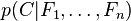
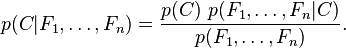
In plain English the above equation can be written as

$\mbox{posterior} = \frac{\mbox{prior} \times \mbox{likelihood}}{\mbox{evidence}}. \,$

关键是计算分子，因为分母为常数

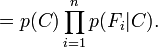
而分子可以展开为

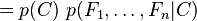
The numerator is equivalent to the joint probability model

$p(C, F_1, \dots, F_n)\,$

which can be rewritten as follows, using repeated applications of the definition of conditional probability:

$p(C, F_1, \dots, F_n)\,$

$= p(C) \ p(F_1,\dots,F_n\vert C)$

$= p(C) \ p(F_1\vert C) \ p(F_2,\dots,F_n\vert C, F_1)$

$= p(C) \ p(F_1\vert C) \ p(F_2\vert C, F_1) \ p(F_3,\dots,F_n\vert C, F_1, F_2)$

$= p(C) \ p(F_1\vert C) \ p(F_2\vert C, F_1) \ p(F_3\vert C, F_1, F_2) \ p(F_4,\dots,F_n\vert C, F_1, F_2, F_3)$

$= p(C) \ p(F_1\vert C) \ p(F_2\vert C, F_1) \ p(F_3\vert C, F_1, F_2) \ \dots p(F_n\vert C, F_1, F_2, F_3,\dots,F_{n-1}).$

Now the "naive" conditional independence assumptions come into play: assume that each feature F_i is conditionally independent of every other feature F_j for $j\neq i$ . This means that

$p(F_i \vert C, F_j) = p(F_i \vert C)\,$

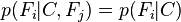
for $i\ne j$ , and so the joint model can be expressed as

$p(C, F_1, \dots, F_n) = p(C) \ p(F_1\vert C) \ p(F_2\vert C) \ p(F_3\vert C) \ \cdots\,$

$= p(C) \prod_{i=1}^n p(F_i \vert C).\,$

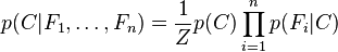
This means that under the above independence assumptions, the conditional distribution over the class variable C can be expressed like this:这里是最终的分子：

$p(C \vert F_1,\dots,F_n) = \frac{1}{Z} p(C) \prod_{i=1}^n p(F_i \vert C)$

Constructing a classifier from the probability model

The discussion so far has derived the independent feature model, that is, the naive Bayes probability model. The naive Bayes classifier combines this model with a decision rule. One common rule is to pick the hypothesis that is most probable; this is known as the maximum a posteriori or MAP decision rule. The corresponding classifier is the function classify defined as follows:贝叶斯分类器的构造，通常为使用最大似然优化以下函数

$\mathrm{classify}(f_1,\dots,f_n) = \underset{c}{\operatorname{argmax}} \ p(C=c) \displaystyle\prod_{i=1}^n p(F_i=f_i\vert C=c).$

更详细的判别函数，及参数估计（最大似然及贝叶斯参数估计）的推导最好看书，推荐《模式分类》