▶ 回归问题的提升树,采用分段常数函数进行回归,每次选择一个分界点及相应的两侧估值,最小化训练数据在两侧的残差平方和的和,然后将当前残差作为下一次训练的数据,最后把各次得到的分段函数加在一起,就是最终回归结果
● 代码
 1 import numpy as np
 2 import matplotlib.pyplot as plt
 3 from matplotlib.patches import Rectangle
 4
 5 trainDataRatio = 0.3
 6 dataSize = 1000
 7 defaultEpsilon = 0.05                                                           # 需要进行分段的最小区间宽度
 8 randomSeed = 103
 9
10 def myColor(x):                                                                 # 颜色函数
11     r = np.select([x < 1/2, x < 3/4, x <= 1, True],[0, 4 * x - 2, 1, 0])
12     g = np.select([x < 1/4, x < 3/4, x <= 1, True],[4 * x, 1, 4 - 4 * x, 0])
13     b = np.select([x < 1/4, x < 1/2, x <= 1, True],[1, 2 - 4 * x, 0, 0])
14     return [r**2,g**2,b**2]
15
16 def dataSplit(dataX, dataY, part):                                              # 将数据集分割为训练集和测试集
17     return dataX[:part],dataY[:part], dataX[part:], dataY[part:]
18
19 def judgeStrong(x, para):                                                       # 强分类判别函数,调用弱分类判别函数进行线性加和
20     return para[1][targetIndex(x, para[0])]
21
22 def targetIndex(x, xList):                                                      # 二分查找 xList 中大于 x 的最小索引
23     lp = 0
24     rp = len(xList) - 1
25     while lp < rp - 1:
26         mp = (lp + rp) >> 1
27         if(xList[mp] >= x):
28             rp = mp
29         else:
30             lp = mp
31     return rp
32
33 def createData(count = dataSize):                                               # 创建数据
34     np.random.seed(randomSeed)
35     X = np.random.rand(count)
36     Y = X * (32 / 3 * (X-1) * (X-1/2) + 1)
37     return X, Y
38
39 def adaBoost(dataX, dataY, weakCount):                                          # 提升训练
40     count = len(dataX)
41     xSort, ySort = zip( *sorted(zip(dataX, dataY)) )
42     xSort = np.array(xSort)
43     ySort = np.array(ySort)
44
45     result = np.zeros([weakCount,3])
46     for i in range(weakCount):
47         table = np.zeros(count - 1)
48         for j in range(count - 1):                                              # 找最佳分割点,损失函数为两侧残差平方和的和
49             #table[j] = np.sum( (ySort[:j+1] - np.mean(ySort[:j+1]))**2 ) + np.sum( (ySort[j+1:] - np.mean(ySort[j+1:]))**2 )
50             table[j] = -np.sum(ySort[:j+1])**2 / (j+1) - np.sum(ySort[j+1:])**2 / (count - j - 1)    # 简化一点计算量
51         index = np.argmin(table)
52
53         valueLeft = np.mean(ySort[:index+1])                                    # 两侧估值
54         valueRight = np.mean(ySort[index+1:])
55         result[i] = np.array([ xSort[index], valueLeft, valueRight ])           # 当前结果暂存,表示当前分类器以 xSort[index] 为分点,左右侧取值分别为 valueLeft 和 valueRight
56         ySort[:index+1] -= valueLeft                                            # 两侧新残差
57         ySort[index+1:] -= valueRight
58
59     result = np.array(sorted(result, key=lambda x:x[0]))
60     #L = np.triu( np.tile(result[:,1], [weakCount+1,1]), 0 )                         # 分段结果加和为最终分类器,注意段数为 weakCount + 1
61     #R = np.tril( np.tile(result[:,2], [weakCount+1,1]), -1)                         # 这里第 i 行 等于 r[0] + r[1] + ... + r[i-1] + l[i] + l[i+1] + ... +l[n],表示第 i 个分点
62     #return np.concatenate(( result[:,0], np.array([np.inf]) )), np.sum(L + R, 1)    # 其中第 0 行是 np.sum(result[:,1]),第 weakCount 行是 np.sum(result[:,2])
63     L = np.concatenate((                  np.cumsum(result[:,1].T[::-1])[::-1], np.array([0.0]) )) # 简化一点计算量和空间开销
64     R = np.concatenate(( np.array([0.0]), np.cumsum(result[:,2].T) ))
65     return np.concatenate(( result[:,0], np.array([np.inf]) )), L + R
66
67 def test(weakCount):                                                            # 单次测试
68     allX, allY = createData()
69     trainX, trainY, testX, testY = dataSplit(allX, allY, int(dataSize * trainDataRatio))
70
71     para = adaBoost(trainX, trainY, weakCount)
72
73     testResult = [ judgeStrong(i, para) for i in testX ]
74     errorRatio = np.sum( np.abs(np.array(testResult) -  testY) ) / (dataSize*(1-trainDataRatio))
75     print( "weakCount = %d, errorRatio = %f"%(weakCount, round(errorRatio,4)) )
76
77     fig = plt.figure(figsize=(10, 8))                                           # 画图
78     plt.xlim(-0.1, 1.1)
79     plt.ylim(-0.1, 1.1)
80     XX = [0.0] + para[0][:-1].flatten().tolist() + [1.0]
81     YY = [ judgeStrong(i, para) for i in XX ]
82     plt.scatter(testX, testY, color = myColor(1), s = 8, label = "originalData")
83     for i in range(weakCount+1):
84         plt.plot(XX[i:i+2], [YY[i+1], YY[i+1]],color = myColor(0), label = "regressionData")
85     plt.text(0.1, 1.0, "weakCount = " + str(weakCount) + "
errorRatio = " + str(round(errorRatio,4)), size = 15, ha="center", va="center", bbox=dict(boxstyle="round", ec=(1., 0.5, 0.5), fc=(1., 1., 1.)))
86     R = [ Rectangle((0,0),0,0, color = myColor(1 - i)) for i in range(2) ]
87     plt.legend(R, ["originalData", "regressionData"], loc=[0.79, 0.012], ncol=1, numpoints=1, framealpha = 1)
88
89     fig.savefig("R:\weakCount" + str(weakCount) + ".png")
90     plt.close()
91
92 if __name__ == '__main__':
93     test(1)
94     test(2)
95     test(3)
96     test(4)
97     test(20)
98     test(100)
● 输出结果,包含训练轮数和预测错误率
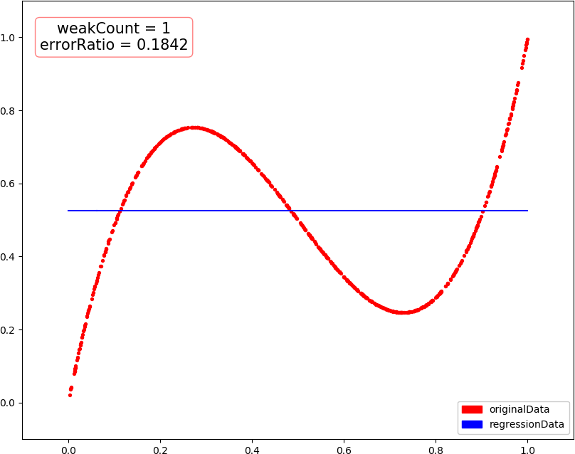
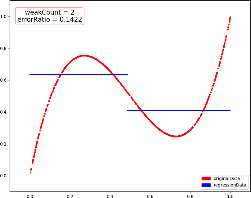
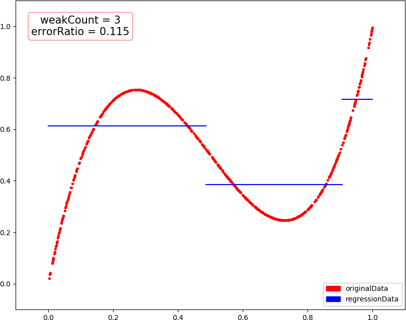
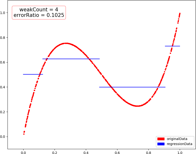
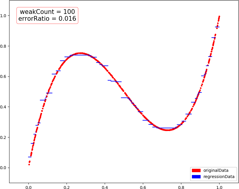
weakCount = 1, errorRatio = 0.184200
weakCount = 2, errorRatio = 0.142200
weakCount = 3, errorRatio = 0.115000
weakCount = 4, errorRatio = 0.102500
weakCount = 20, errorRatio = 0.035300
weakCount = 100, errorRatio = 0.016000
● 画图,总数据量 1000,训练集 300,测试集 700

● 画图,当总数据量减为 500,训练集 150 时,出现了过拟合?
