GISOO通信--
https://github.com/araujokth/kth-gisoo/wiki/Installing-GISOO
简介
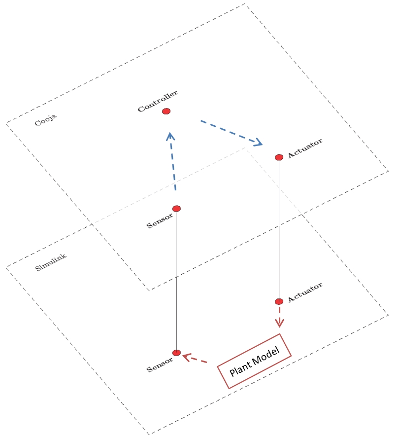
GISOO代表Simulink和COOja的图形集成,并且名称代表GISOO中的每个模拟应该包括两个模拟的组合,一个在Cooja中,另一个在Simulink中,它们与数据通信的可能性同步。事实上,所有无线系统(也可以包含控制器)都将在Cooja中进行模拟,系统将在Simulink中进行模拟,每当Cooja中的模拟系统需要测量系统中的某些变量或在那里驱动一些执行器时,传感器Cooja中的执行器或执行器将发送传感器值请求或将驱动数据发送到Simulink模型中与镜像模型接触的镜像传感器或执行器,它们可以接收所请求的传感器数据或应用驱动值。下图显示了GISOO的一般视图,它可以显示Cooja和Simulink中的镜像元素以及与植物相关的微粒的位置。 (下图显示了控制器位于其中一个控件中的情况,但也可以将控制器放在PC中)
为了使上述系统工作,我们需要能够进行适当的数据通信,并且两个系统都应该同步工作。因此,创建GISOO的主要事实是提供适当的数据通信系统和准确的同步。以下部分将说明为实现这些目标而设计和实施的部件的详细信息。由于数据通信也用于同步,首先我们需要了解数据通信细节。
数据通信
在GISOO中准备模拟的第一步,我们需要将所有无线节点添加到Cooja环境中,然后在下一步中我们需要激活Cooja(GISOO-Simulink插件)中提供的GISOO插件来处理GISOO的数据通信和同步。此插件将创建一个UDP端口,端口号等于“18000 + Mote-id”,它将侦听此端口以接收来自Simulink的与此mote相关的数据。这意味着Cooja中的每个微尘都有自己特定的UDP端口来接收数据。
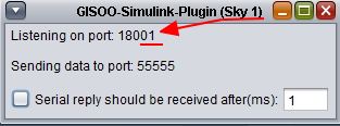
另一方面,Simulink模型有不同的情况,所有模型都将从一个预定义的UDP端口接收数据,默认端口号为55555.这意味着Simulink甚至是Simulink的特定部分应该接收的所有数据模型应该发送到这个端口。
仿真过程
在GISOO中,Cooja负责控制模拟程序。这意味着Cooja将开始模拟无线系统,直到Cooja中的一个节点需要向系统模型发送或从系统模型接收一些数据。这可能发生在四种情况:
- 传感器微尘需要感测一些传感器数据。
- 执行器微尘需要在系统上施加一些作动值。
- 微尘需要发送一些串行数据。
- 微尘需要接收一些串行数据。
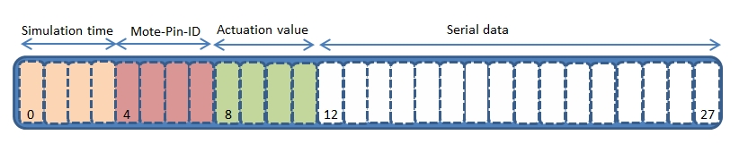
在任何这些情况下,Cooja中的微尘都会向Simulink模型发送一条消息,告知Simulink哪个时刻需要哪种动作。为了实现这一目标,已经设计了特殊的消息结构。此消息包含四个不同部分:
- 模拟时间
- mote-ID
- 驱动值(uValue)
- 串行数据
模拟时间(4个字节):在消息结构中考虑用于承载模拟时间的前四个字节(以毫秒为单位)。事实上,Cooja将运行直到mote需要与Simulink进行特殊通信,然后它将生成一条消息并将Cooja中的模拟时间添加到消息的开头。另一方面,Simulink将暂停模拟,直到收到Cooja的消息。然后在第一步中,它将从消息开始提取Cooja时间,并运行Simulink模拟以达到特定时刻。此过程将在本页的同步说明中进行说明。
Mote-Pin-ID(4字节):每当由Cooja中的微尘生成的消息时,Simulink作为接收者应该知道该消息来自哪个微尘并且应该影响该微尘的哪个部分(引脚)。例如,当id = 4的微尘需要从其ADC1读取数据时,在将被发送到Simulink的消息中,“mote-id”和“ADC1(我们称之为引脚号)”都应该清楚。为此,我们通过此方法创建了一个名为mote-pin-id的数字:
mote-pin-id = Mote-id*100 + pin number
and considered pin-ids are:
- ADC0 - ADC12 = 0 - 12
- DAC0 - DAC1 = 16 - 17
- Serial data to be sent to Simulink = 18
- Serial data to be received from Simulink = 19
执行值(uValue - 4个字节):虽然只有部分消息用于向系统应用激励值,但由于GISOO中需要修复消息格式,这四个字节将在所有消息中,但这些字节只有当Cooja中的微尘想要对系统施加驱动值时,它们才会获得价值。
串行数据(16字节):出于与启动值相同的原因,所有消息都将携带16字节的串行消息,但只有在需要将某些串行数据从Cooja传输到Simulink或其中时才会使用它们。反之亦然。
下图显示了GISOO的设计消息结构的模式。
同步
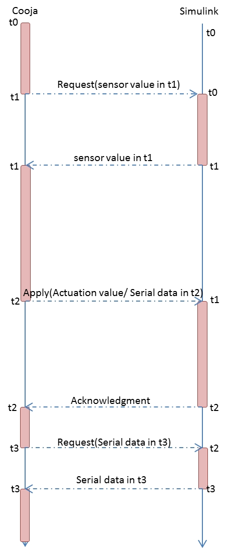
GISOO的另一个重要因素是其精确的同步系统。在已提到的GISOO中,Cooja将控制模拟时间,因此Cooja将运行其模拟,直到Cooja中的微尘需要向Simulink发送或从Simulink接收一些数据。在这一刻,Cooja中用于该mote的GISOO插件将创建一条消息并将其发送到Simulink,其中包含Cooja中的准确模拟时间(以毫秒为单位)。一旦插件发送消息,它将在那一刻暂停模拟以接收来自Simulink的回复。此回复可以是传感器值或串行数据或确认,但接收数据很重要,否则Cooja将不会继续其模拟。 Cooja中的暂停始终通过在发送数据后执行“接收”命令来创建。由于“接收”命令是阻塞功能,因此模拟将保持该时刻,直到它可以读取某些数据并通过该状态。以下代码显示了代码的一部分,该代码发送ADC值请求并在模拟中暂停,直到接收到该时刻的ADC。
另一方面,Simulink从一开始就处于暂停模式,它会等到收到来自Cooja的消息。一旦收到消息,它将在Cooja中提取模拟时间,然后它将继续模拟,直到它到达Cooja中的模拟时间,然后发回所请求的数据或在那一刻应用驱动数据。两条消息之间的持续时间是Simulink可以独立于Cooja模拟运行模拟的持续时间,因为通常Simulink比Cooja快得多,Simulink可以在很短的时间内捕获Cooja中的模拟时间。取决于Simulink中系统模型的复杂性。下图显示了GISOO中同步和消息通信的组合。
GISOO Simulink library
GISOO使用其特定的Simulink库,这部分将解释设计系统的细节,以实现模拟中的正确功能。
GISOO仿真环境
GISOO-Simulink-library包含一个主块,用于处理同步和数据通信(在Simulink中接收数据),称为“GISOO-Simulation Environment”。这个模块模拟了Simulink中的Cooja环境及其内容,如果我们需要在Simulink中实现控制器模型,它应该被添加到这个模块中。系统模型应位于此区块之外。在这里和这里可以找到更多的解释和例子。 “GISOO-Simulation Environment”块是一个do-while块,它可以暂停模拟系统模型“while”它没有收到Cooja的新时间,并且在收到来自Cooja的模拟时间后“do”继续模拟系统模型
该块也应该能够连续接收来自Cooja的消息,为此我们添加了可以处理接收数据的附加部分。下图显示了“GISOO_Simulation_Environment”块。

“GISOO_Simulation_Environment”内部如下图所示。如图所示,它包含一个GISOO-Simulink插件块,负责从Cooja接收数据,并且它将同步Simulink和Cooja。另一个块是“SynchronizerLoop”,它只控制Simulink中的do while循环。


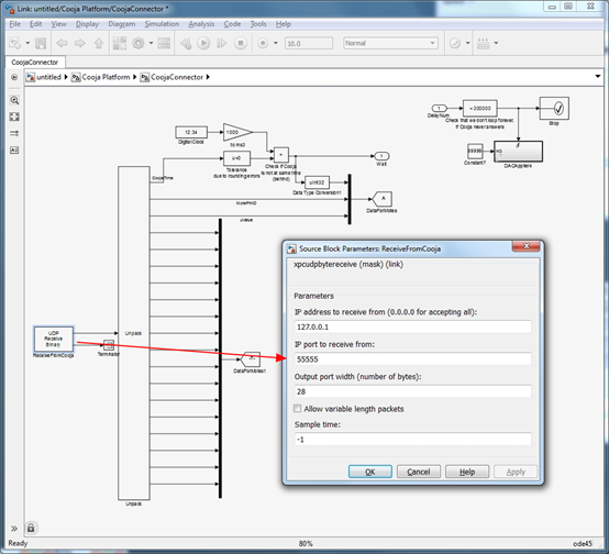
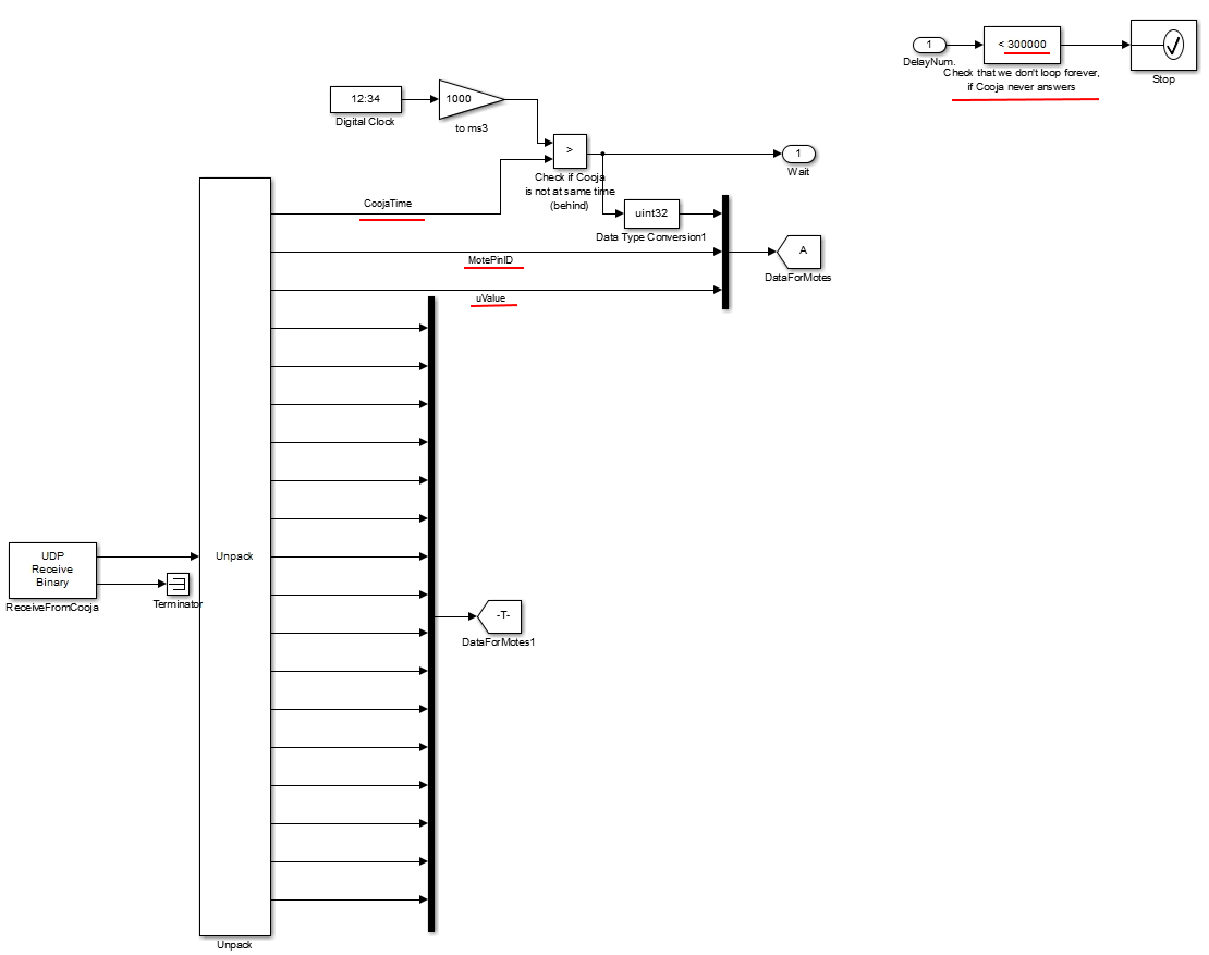
下图显示了整个“GISOO-Simulink插件”。如图所示,该块将从Cooja接收消息并提取Simulation-Time,mote-pin-id,uValue和串行数据,并将Simulink中的Simulation时间与Cooja中的Simulation时间进行比较,如果是Simulink落后,它将继续模拟到达适当的时间。图片右上角的三个块显示了while循环将执行的最大迭代次数。此数字将配置Simulink可以等待从Cooja接收消息的最长时间,如果Simulink在此期间未收到任何消息,则会将其视为与Cooja通信时出现问题的结果,并避免不确定的模拟循环,停止块将停止Simulink Simulation,它将在屏幕上显示一条消息。 (如果在场景中你需要更大的时间间隔来接收来自Cooja的消息,你可以增加该块的默认值,在下图中为300000。)
下图显示了Stop块在达到其最大迭代次数之前无法从Cooja接收消息时创建的消息。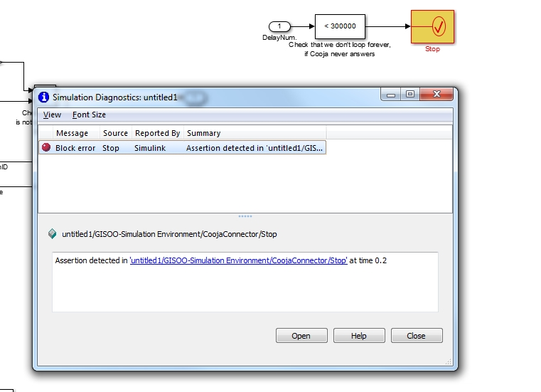
SKY-mote
SkyMote bloke旨在模仿真实微尘的动作,例如读取ADC,在DAC上写入以及在Simulink中发送和接收无线电数据。下图显示了SkyMote块的结构。该块将从“GISOO-Simulation-Environment”中的“CoojaConnector”块接收四个数据:
- Time-Is-Correct:是一个布尔值,表示Simulink时间是否等于从消息收到的 Cooja时间。
- 接口标识符:mote-pin-id的值,已在数据通信中进行了解释
- uValue:是DAC的驱动值,它也在数据通信中得到了解释
- 输入串行数据:是从Cooja接收的串行数据。
除了上述值之外,SkyMote还可以从mote输入接收输出串行数据。
在mote结构图中,左边的第一个彩色列(浅橙色)是代表motes的pin-id的常数块。 pin-id的值已在数据通信中解释。这些值将用于找出接收的数据属于哪个引脚。
其他三个彩色列是三个过滤器,最终可以根据接收的数据在微尘中做出正确的动作。
左侧的第一个过滤器列以浅绿色显示,将发现接收到的pin-id是否与已比较的常数相同。对于Simulink中收到的每条消息,这些块中只有一个将返回true,其余块将为false。
在第二次比较中,首先从mote-pin-id值中提取mote-id的值,然后将该值与Simulink中的mote的id进行比较。如果比较的结果为真,则表示收到的消息属于此mote,否则它属于某些其他节点。在最后一步中,我们将“比较”(逻辑和)此比较的布尔结果与前一个过滤器的结果,并且此AND可以被视为已在橙色列中显示的第二层过滤。
最后,最后一个过滤器将检查Simulink中的模拟时间是否与我们在收到的消息中收到的Cooja中的模拟时间完全相同。此步骤也将通过在GISOO-Simulink插件(IsTimeCorrect)中执行第二个过滤器的结果和接收到的布尔值之间的逻辑AND来实现,并创建在图片中以黄色显示的第三个和最后一个过滤器。只有能够通过滤波器所有这些层的数据才能激活正确的动作块,该动作块将执行ADC读取或应用DAC值或接收串行数据或发送串行数据。由于我们总是使用ADC0和ADC1,我们只使用它们,我们在块模型中终止其余的ADC。但它们可以在需要的情况下使用。 (ADC5应该是活动的但是没有使用,因为Cooja中有一些未经研究的问题。)
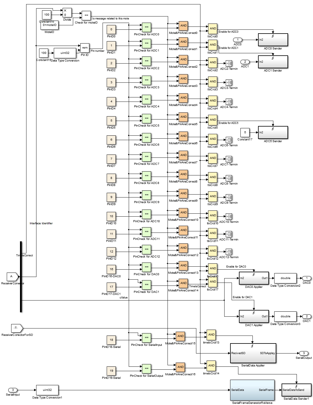
需要额外程序的唯一操作是发送串行数据。因为当我们想要将数据发送到mote的串行端口时,我们应该创建一个完整的串行消息,包括它的头,有效负载(串行数据)和页脚,在这个模型中我们也传递了来自专门设计的块的串行数据创建一个串行消息。(该块在上图中以浅蓝色显示)串行消息的结构可以在TEP 113中找到。但应该提到的是,CRC的两个字节应该在P上创建结束有效载荷。 (在TEP-113结束时提到的有效载荷结束之前不会超过S)
How to use GISOO
How to use GISOO · araujokth/kth-gisoo Wiki · GitHub
Overview
GISOO is an integration of Simulink and COOJA for performing simulation of wireless cyber-physical systems. Thus, each part of the wireless cyber-physical system can be implemented as follows:
- the physical system model is implemented in Simulink.
- the wireless sensors, actuators and relays (from physical layer to application layer) are emulated in COOJA
- the estimator/controller can be implemented in either a wireless node in COOJA, or emulated in a CPU in Simulink. The implementation in Simulink allows for a faster design and evaluation since no recompilation of wireless nodes code is necessary.
One of our main goals is codeyou upload to the real wireless nodes for performing a real experiment. For this to be achieved, GISOO provides the following interfaces:
- Analog-to-digital converter (ADC), for interfacing wireless nodes with real sensors
- Digital-to-analog converter (DAC), for interfacing wireless nodes with real actuators
- Serial interface, for allowing communication to sensor, actuators and processing units (CPUs, embedded computers, microcontrollers, etc).
In this section you can find all the information on how to use GISOO and a simple example which can help you build your own applications from.
Note: As standard in the wireless sensor network literature, we will the terms wireless node, wireless mote, wireless sensor node or simply node or mote to mean a low-rate wireless device communicating using a IEEE 802.15.4 radio.
Compiling your wireless node code
First, you should compile the code which you want to upload to your wireless nodes. You can either use TinyOS code or Contiki code for your applications. However, we remind you that at the moment all our examples are based on TinyOS.
In TinyOS you compile your application in a wireless node by executing for eaxmple: "make telosb" for a telosb/tmote sky/cm5000 device. When you do such operation, a "build" folder is automatically created in the application folder, which contains some files including the "main.exe". This file will be used in COOJA as the mote application. You can find a TinyOS installation manual here and also check TinyOS tutorials For more detail about its commands.
Note that you can load several distinct wireless nodes with different applications in the same COOJA simulation.
COOJA setup
In order to use GISOO, we must start COOJA, create a new simulation and include the required wireless nodes. Particularly, we must connect the sensors, actuators and all of the wireless nodes which have a direct interface to Simulink. For example, a sensor is likely to take ADC measurements from the physical system (Simulink model), and an actuator is likely to send a control signal (either DAC or serial communication) to the actuator which affects the physical system. We explain these steps below.
COOJA Execution
Note: We now present the execution details in a Windows system, however, we note that the execution for a Linux system is identical. The only difference comes from the fact that Cygwin is used in the Windows system, while the terminal is used in the Linux system
For executing COOJA, open a shell window of Cygwin and navigate to COOJA's directory. In this example, Cygwin has been installed at C:cygwin and the Contiki folder which contains COOJA, is located at C:contiki-2.6. This step is shown in the screenshot below. Finally in the COOJA's folder you should use execute “ant run” command to run COOJA.

Create a new simulation
To start a new simulation, create a new simulation environment by going to the file menu as shown in the picture:

In the window of new simulation creation, you can select a name for your simulation and select your desired radio medium. You can also select the random seed for your simulation, which should be always the same if you want to perform exactly the same simulation every time. The "Create new simulation" window is shown below:

After following these steps, the new simulation environment will be created which will result in the following:

Adding motes to the simulation
After creating the new simulation environment you have to add all the wireless nodes to the simulation. Although COOJA supports different types of nodes and operating systems, we used the Sky Mote (MSP430-based node) and TinyOS in all of our experiments. However, one can simulate nodes using both Contiki OS and TinyOS at the same time in COOJA.
In order to add a new mote to the simulation you can use the Motes menu and navigate to "Motes>Add motes>Create new mote type>Sky mote" as shown in the following image:

In the opened window you should follow these steps:
- Select a name for you mote
- Use the browse button to find the "main.exe" of the application that you want to load in your mote
- Create the mote
These steps are shown in the following image:

After selecting the "main.exe" and creating the mote, the next window will ask you about the number of desired motes from that application and the location of the motes which by default will be selected randomly.

You can repeat this procedure for all nodes and all different applications you would like to simulate.
Finally, after the previous procedure, the virtual mote will be created.
Note that the number which has been appeared on each mote is its mote-id and it has been selected automatically (in-order) which is not configurable by the user. This is important to remember since in many applications each nodes operation will depend on their node-id. For these type of scenarios you should create motes in an order that each mote receive your desired id.

Activating the GISOO COOJA Plug-in
In order to connect motes in COOJA to Simulink you need to use the GISOO COOJA plug-in which you have previously downloaded from here and added to your COOJA folder (this has been explained in the installation procedure)
In order to use this plug-in, when running COOJA for the first time, you need to select and activate the plug-in in the COOJA extension list which you can reach and select in "Setting-> COOJA extensions", as depicted in the next image:

Executing the GISOO COOJA plug-in
In each wireless node which interfaces with Simulink (reads data from it, or writes data to it), you have to right click on that mote and select "Mote tools Sky -> GISOO COOJA plug-in". This plugin allows the communication between the mote in COOJA and the virtual mote in Simulink. You can see the procedure in the next image:

As seen in the previous image, GISOO COOJA plug-in is created for the selected mote. The same node-id is created for both the mote in COOJA and the virtual mote in Simulink.

Simulink setup
To follow these steps it is assumed that the GISOO Simulink Library was added already to MATLAB. Now you have access to all the component which you need to be able to run your simulation with GISOO.
Start by creating a new model from MATLAB by going to "File>New>Model", in order to open Simulink. Now in your model window, go to "View>Library Browser" and you should be able to see the GISOO Library and shown in the following image:

Adding the GISOO Simulink Environment (GSE)
The first step in order to perform the simulation is to add the "GISOO Simulink Environment" (GSE) block to your simulation environment. This block is the place that allows for GISOO simulations to take place and where the interface between Simulink and COOJA takes place. It will contain all the necessary virtual motes and also handle the synchronization and communication between Simulink and COOJA. The next image shows the GSE block.

Adding a mote to the GSE
In the next step, the necessary motes are be added inside the GSE block. This can be performed by double clicking on the GSE block and drag a "SkyMote" block from the "GISOO Library" to the GSE block.
Note that on the first attempt to add a mote inside the GSE you may face a message which asks you to disable the link to the library and it should be done by clicking on the "disable" part in the pop-up message, as it has shown in the following picture. If you did not see this message you can just add your mote inside the GSE without any concern.

Finally, you should add all the motes which were enabled with GISOO COOJA Plug-in in COOJA to the GSE. Thus, all nodes that need to be in contact with the plant such as wireless sensors or wireless actuators or other motes which interface with computing nodes in Simulink (e.g., through serial communications), such as a controller implemented in Simulink, should be added to the GSE.
After adding all the virtual nodes to this environment, it is necessary to set their node-id by double clicking on them. This number should be set to the same id of their mirror motes in COOJA. As expected, GISOO only allows for a mote in Simulink to communicate with the mote in COOJA if both have the same node-id.

Adding ADC/DAC connectors
For each node, according to its action you should add the required ADC or DAC connector component. For instance if you have added a mote to operate as a sensor which should measure data on the ADC0 pin (input to the node), then you have to connect the ADC-Connector component to ADC0 input of that mote, or if you want to receive some actuation data on the DAC0 (output of the node), you need to add the DAC connector component on the DAC0 output of your mote. These components and their location is shown in the following picture.

Adding the plant/physical system model
In the final step, we need to add a physical model of our plant which can be modeled in a Discrete State-Space block outside the GSE. We now have a different number of input and output from our GSE block, which has been created by the ADC-connector or DAC-connector components from the previous step.
Now in this step the outputs from the GSE should be used as the input for our plant model and the output of the plant model should be used as the input for the "GISOO-Simulation Environment". The following picture shows a simple environment and the interaction between the GSE and the plant model.

Configuration and running the simulation
After preparing the simulation environment for the very last configuration, you have to setup the Simulink simulation to act in a fix-step instead of variable-step. You can apply this configuration in the "Configuration parameter" window which is accessible from "Simulation->Model Configuration Parameter" and finally change the type in the solver option to the fix-step. Now you can select the size of the sample time which we usually configure to "0.001" s to have an accuracy of one millisecond (1 ms).

Now that both sides of the simulation environment(COOJA and Simulink) have been configured we are ready to run the simulation. We have to first start the simulation in Simulink and then start the COOJA simulation. In this step first Simulink will start its simulation for very first milliseconds and then it will wait until it receives any incoming data from COOJA. The only important point in this action is that if Simulink cannot receive the message from COOJA in less than few seconds it will consider it as a problem and will go out from the simulation execution loop, so it is necessary to run the COOJA in few second after Simulink.
Simple Scenario
We now present an example of a closed-loop control experiment in GISOO.
The wireless double-tank system is shown in the next figure. Water is pumped from a reservoir to the upper tank, from which it flows through an outlet to the lower tank. Water from the lower tank flows through a similar outlet back to the reservoir. The pump is controlled by an actuation signal, which is a control voltage applied to the pump motor. The water levels in both tanks are measured using pressure sensors.
For sensing and actuation we use sky wireless nodes. These motes contain ADCs (analog-to-digital converters) and DACs (digital-to-analog converters), which are used to connect to the sensors and actuators in the physical system.
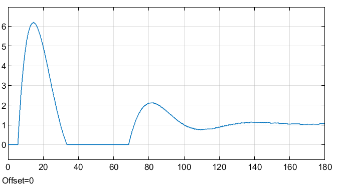
The aim of this scenario is to create such a system which can stabilize the water level in the lower tank on constant level (in this example, the level is set to 5cm). The system is composed of 4 different devices:
-
Sensor Node: A sky node is connected to the pressure sensors from the tank process, and takes measurements using the ADC and transmits this information to the Relay node.
-
Relay Node: Another node is programmed to relay messages between the Sensor Node and the Controller Node. This introduces multi-hop communications.
-
Controller Node: The control algorithm is implemented inside the wireless node. This node receives measurements from the Relay Node, computes the actuation value and transmits an appropriate control action to the Actuator Node.
-
Actuator Node: Another node is connected to the pump motor using the DAC. This node receives the control signal from the controller and applies this voltage to the pump in the tank setup.
For this sample, you can download the prepared codes for these motes from here.

In order to create such a system in GISOO we have to:
- Create all the nodes in COOJA
- Enable the GISOO COOJA plug-in in the nodes which interface the plant
- Create a proper GSE in Simulink including all the nodes that interface the plant.
- Finally, we have to make a model of the plant in Simulink and connect it to the GSE.
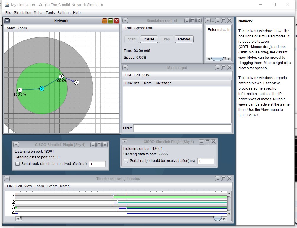
In the first step we have to create a simulation with four nodes, as it is shown in the next figure. In this scenario, each node should have its special id as follows:
- Sensor: 1
- Relay: 2
- Controller: 3
- Actuator: 4
To create motes with these ids, the order of mote creation in COOJA, should be the same as the motes' id.
After adding these nodes, since the sensor should sense the water levels from the plant and the actuator should be able to actuate the plant, both of them should be connected to Simulink. It is then needed to activate the "GISOO COOJA Plug-in" for both of these nodes.

In the next step, you have to create a Simulink model, add a GSE block and add two sky node blocks from the GISOO library. Tese node blocks are the mirror nodes for the Sensor and Actuator in COOJA. Thus, they must have the same node id as the nodes in COOJA. This step is shown in the next figure.

In order to create a model of the plant we can use the "Discrete State-Space(Plant)". For this aim we can write a MATLAB script and add it to the "initFcn" of callbacks in the Model properties.
The required MATLAB script (Simulink model) for this experiment can be downloaded from here.

Finally, the simulation environment is ready and you can run the simulation by running Simulink first, followed by starting COOJA.
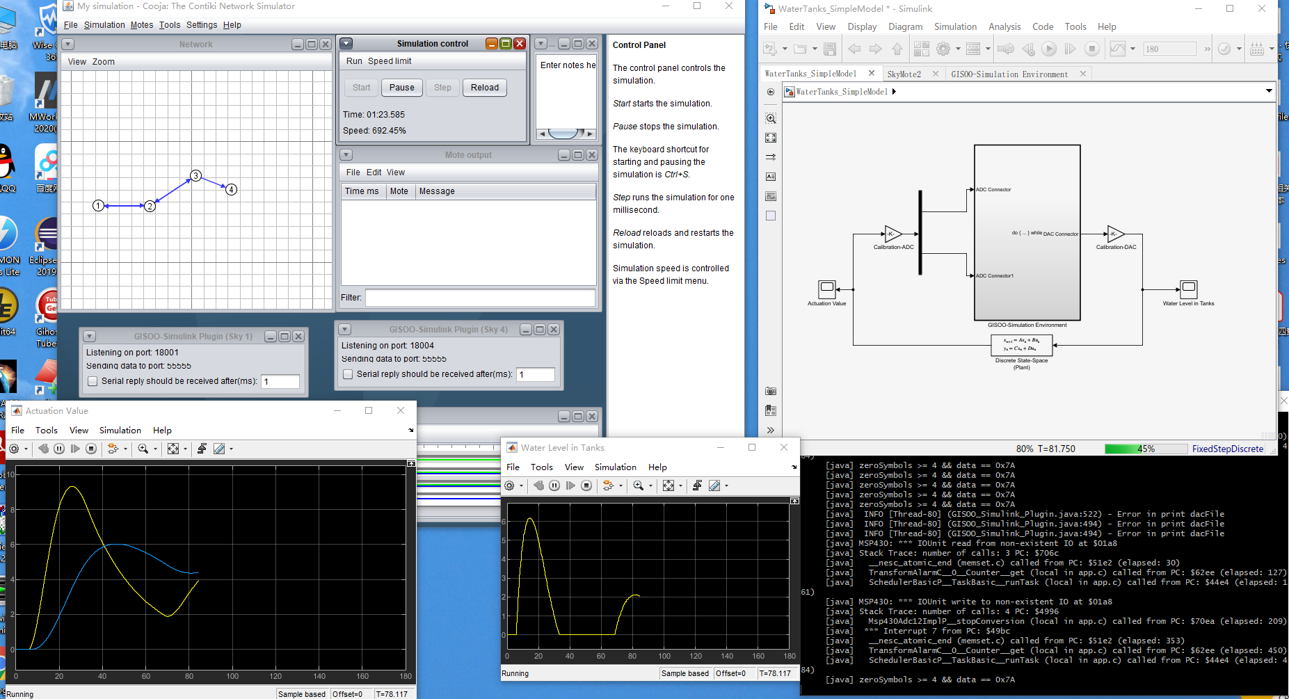
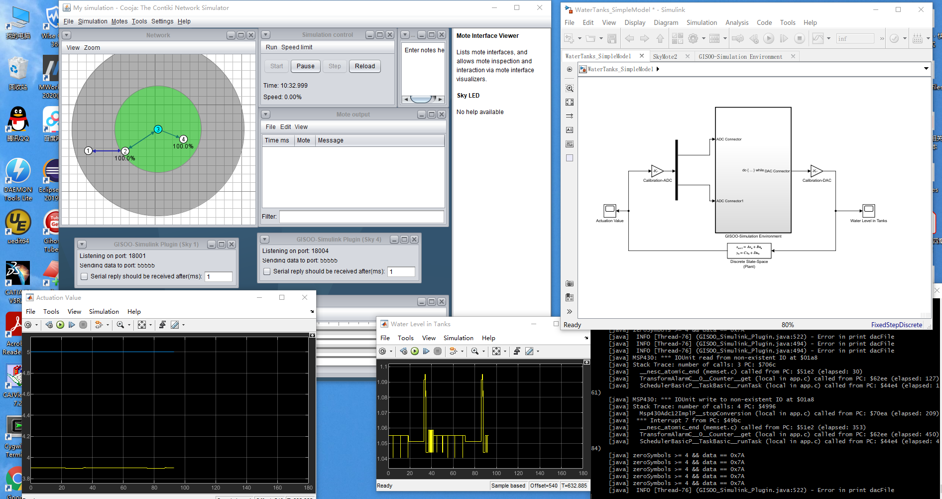
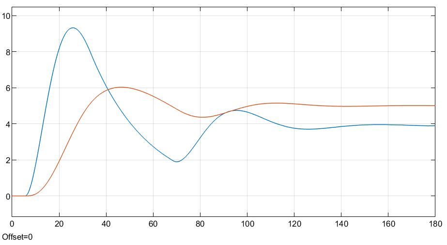
Although you can save all data from Simulink or COOJA for further analyzes, you may also monitor online the signals in both simulators. The next two figures show the changes in the water levels and actuation values during the experiments happening online.


You can download all of the required codes (node codes, plant script, and Simulink model) from here. Then you just need to create the COOJA simulation and run the simulation!
自己实际的操作演示:
截图过程

最后一次打开了! 重新打开看看!
windows 10 cygwin64 contiki2.6 tinyos
matlab 2018b