几个有助于加深对反向传播算法直观理解的网页,包括普通前向神经网络,卷积神经网络以及利用BP对一般性函数求导
A Visual Explanation of the Back Propagation Algorithm for Neural Networks
Let's assume we are really into mountain climbing, and to add a little extra challenge, we cover eyes this time so that we can't see where we are and when we accomplished our "objective," that is, reaching the top of the mountain.
Since we can't see the path upfront, we let our intuition guide us: assuming that the mountain top is the "highest" point of the mountain, we think that the steepest path leads us to the top most efficiently.
We approach this challenge by iteratively "feeling" around you and taking a step into the direction of the steepest ascent -- let's call it "gradient ascent." But what do we do if we reach a point where we can't ascent any further? I.e., each direction leads downwards? At this point, we may have already reached the mountain's top, but we could just have reached a smaller plateau ... we don't know. Essentially, this is just an analogy of gradient ascent optimization (basically the counterpart of minimizing a cost function via gradient descent). However, this is not specific to backpropagation but just one way to minimize a convex cost function (if there is only a global minima) or non-convex cost function (which has local minima like the "plateaus" that let us think we reached the mountain's top). Using a little visual aid, we could picture a non-convex cost function with only one parameter (where the blue ball is our current location) as follows:

Now, backpropagation is just back-propagating the cost over multiple "levels" (or layers). E.g., if we have a multi-layer perceptron, we can picture forward propagation (passing the input signal through a network while multiplying it by the respective weights to compute an output) as follows:

And in backpropagation, we "simply" backpropagate the error (the "cost" that we compute by comparing the calculated output and the known, correct target output, which we then use to update the model parameters):

It may be some time ago since pre-calc, but it's essentially all based on the simple chain-rule that we use for nested functions

Instead of doing this "manually" we can use computational tools (called "automatic differentiation"), and backpropagation is basically the "reverse" mode of this auto-differentiation. Why reverse and not forward? Because it is computationally cheaper! If we'd do it forward-wise, we'd successively multiply large matrices for each layer until we multiply a large matrix by a vector in the output layer. However, if we start backwards, that is, we start by multiplying a matrix by a vector, we get another vector, and so forth. So, I'd say the beauty in backpropagation is that we are doing more efficient matrix-vector multiplications instead of matrix-matrix multiplications.
From UFLDL tutorial
Introduction
In the section on the backpropagation algorithm, you were briefly introduced to backpropagation as a means of deriving gradients for learning in the sparse autoencoder. It turns out that together with matrix calculus, this provides a powerful method and intuition for deriving gradients for more complex matrix functions (functions from matrices to the reals, or symbolically, from  ).
).
First, recall the backpropagation idea, which we present in a modified form appropriate for our purposes below:
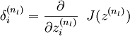
- For each output unit i in layer nl (the final layer), set
- For

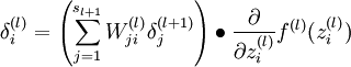
- For each node i in layer l, set
- For each node i in layer l, set
- Compute the desired partial derivatives,

Quick notation recap:
- l is the number of layers in the neural network
- nl is the number of neurons in the lth layer
 is the weight from the ith unit in the lth layer to the jth unit in the (l + 1)th layer
 is the input to the ith unit in the lth layer
 is the activation of the ith unit in the lth layer
 is the Hadamard or element-wise product, which for
  matrices A and B yields the matrix
  such that
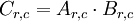
- f(l) is the activation function for units in the lth layer
Let's say we have a function F that takes a matrix X and yields a real number. We would like to use the backpropagation idea to compute the gradient with respect to X of F, that is  . The general idea is to see the function F as a multi-layer neural network, and to derive the gradients using the backpropagation idea.
To do this, we will set our "objective function" to be the function J(z) that when applied to the outputs of the neurons in the last layer yields the value F(X). For the intermediate layers, we will also choose our activation functions f(l) to this end.
Using this method, we can easily compute derivatives with respect to the inputs X, as well as derivatives with respect to any of the weights in the network, as we shall see later.
Examples
To illustrate the use of the backpropagation idea to compute derivatives with respect to the inputs, we will use two functions from the section onsparse coding, in examples 1 and 2. In example 3, we use a function from independent component analysis to illustrate the use of this idea to compute derivates with respect to weights, and in this specific case, what to do in the case of tied or repeated weights.
Example 1: Objective for weight matrix in sparse coding
Recall for sparse coding, the objective function for the weight matrix A, given the feature matrix s:

We would like to find the gradient of F with respect to A, or in symbols,  . Since the objective function is a sum of two terms in A, the gradient is the sum of gradients of each of the individual terms. The gradient of the second term is trivial, so we will consider the gradient of the first term instead.
The first term,  , can be seen as an instantiation of neural network taking s as an input, and proceeding in four steps, as described and illustrated in the paragraph and diagram below:
- Apply A as the weights from the first layer to the second layer.
- Subtract x from the activation of the second layer, which uses the identity activation function.
- Pass this unchanged to the third layer, via identity weights. Use the square function as the activation function for the third layer.
- Sum all the activations of the third layer.

The weights and activation functions of this network are as follows:
| Layer | Weight | Activation function f |
|---|---|---|
| 1 | A | f(zi) = zi (identity) |
| 2 | I (identity) | f(zi) = zi − xi |
| 3 | N/A |  |
To have J(z(3)) = F(x), we can set  .
.
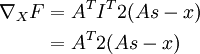
Once we see F as a neural network, the gradient becomes easy to compute - applying backpropagation yields:
| Layer | Derivative of activation function f' | Delta | Input z to this layer |
|---|---|---|---|
| 3 | f'(zi) = 2zi | f'(zi) = 2zi | As − x |
| 2 | f'(zi) = 1 |  |
As |
| 1 | f'(zi) = 1 |  |
s |
Hence,
Example 2: Smoothed topographic L1 sparsity penalty in sparse coding
Recall the smoothed topographic L1 sparsity penalty on s in sparse coding:
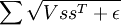
where V is the grouping matrix, s is the feature matrix and ε is a constant.
We would like to find  . As above, let's see this term as an instantiation of a neural network:

The weights and activation functions of this network are as follows:
| Layer | Weight | Activation function f |
|---|---|---|
| 1 | I | |
| 2 | V | f(zi) = zi |
| 3 | I | f(zi) = zi + ε |
| 4 | N/A |  |
To have J(z(4)) = F(x), we can set  .
.
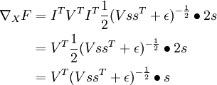
Once we see F as a neural network, the gradient becomes easy to compute - applying backpropagation yields:
| Layer | Derivative of activation function f' | Delta | Input z to this layer |
|---|---|---|---|
| 4 |  |
|
(VssT + ε) |
| 3 | f'(zi) = 1 |  |
VssT |
| 2 | f'(zi) = 1 |  |
ssT |
| 1 | f'(zi) = 2zi | 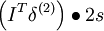 |
s |
Hence,
Example 3: ICA reconstruction cost
Recall the independent component analysis (ICA) reconstruction cost term: 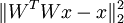 where W is the weight matrix and x is the input.
We would like to find 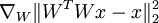 - the derivative of the term with respect to the weight matrix, rather than the input as in the earlier two examples. We will still proceed similarly though, seeing this term as an instantiation of a neural network:

The weights and activation functions of this network are as follows:
| Layer | Weight | Activation function f |
|---|---|---|
| 1 | W | f(zi) = zi |
| 2 | WT | f(zi) = zi |
| 3 | I | f(zi) = zi − xi |
| 4 | N/A | |
To have J(z(4)) = F(x), we can set .
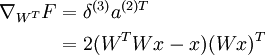
Now that we can see F as a neural network, we can try to compute the gradient  . However, we now face the difficulty that W appears twice in the network. Fortunately, it turns out that if W appears multiple times in the network, the gradient with respect to W is simply the sum of gradients for each instance of W in the network (you may wish to work out a formal proof of this fact to convince yourself). With this in mind, we will proceed to work out the deltas first:
| Layer | Derivative of activation function f' | Delta | Input z to this layer |
|---|---|---|---|
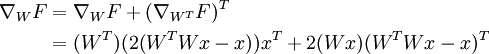
| 4 | f'(zi) = 2zi | f'(zi) = 2zi | (WTWx − x) |
| 3 | f'(zi) = 1 | |
WTWx |
| 2 | f'(zi) = 1 | 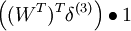 |
Wx |
| 1 | f'(zi) = 1 | 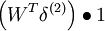 |
x |
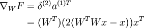
To find the gradients with respect to W, first we find the gradients with respect to each instance of W in the network.
With respect to WT:
With respect to W:
Taking sums, noting that we need to transpose the gradient with respect to WT to get the gradient with respect to W, yields the final gradient with respect to W (pardon the slight abuse of notation here):
Using Computation Graph to Understand and Implement Backpropagation
Recently, by hacking on Assignment2 of the awsome openclass cs231n, I finally stop bumping my head to the wall every time I came across backpropagation, now I even feel a little bit enjoy when hacking the backpropagation process! In this post, I will show how to use computation graph to implement both forward and backward process of Batch Normailzation, Convolution and Pooling.
Batch Normailzation
Bacth Normailzation is a recently proposed method to alleviate the pain in training neural network, especially the special care one needs when initializing weights. Here I won’t go into details to explain the method itself, the details can be found from the paper. But for a quick summary, batch normalization does two things:
- make activation of fully connected or convolutional layer unit gaussian by normalizing the activation
- scale and shift normalized activation so that the network can “choose” to cancel the above step
The algorithm can be summarized like this:

Computation Graph
Building a computation graph is easy, the key is to split operations into basic operations such as add, multiplication or sqrt, but keep in mind don’t split operations too broke, the larger the computation graph, the messier you will feel when backpropagate. The computation graph of Batch Normalization is like this:  The black lines and equations are for the forward pass while the red ones are for the backward pass. Since each gate only completes a simple operation, both the forward pass and backward pass is quite straightfoward. However, special attention might be paid to the summation gate, it confused me for a while. We can see this gate from equation prospect and matrixcodingcoding prospect:

You see, in the forward pass, you sum each row element-wisely to a single row, so each element “contributes” equally to the error. Thus, in the backpropagation pass, you only need to distribute the gradients evenly to rows like the red parts in the graph. Another prospect is to regard this summation as a simple addition like out=row1+row2+...+rowmout=row1+row2+...+rowm, so each rowirowi gets 1 as its local gradient, and you only need to multiply this local gradient with the gradients received by this gate to get row′isrowi′s true gradient.
Feedforward Pass Code
With the computation graph above, the code is quite easy to write:
batch_mean = np.sum(x,axis=0,keepdims=True) / N
batch_var = np.sum((x - batch_mean) ** 2,axis=0,keepdims=True) / N

x_minus_mu = x - batch_mean
ivar = 1.0 / np.sqrt(batch_var+eps)
x_hat = x_minus_mu * ivar
out = gamma * x_hat + beta
running_mean = momentum * running_mean + (1 - momentum) * batch_mean
running_var = momentum * running_var + (1 - momentum) * batch_var
cache = (gamma,x,batch_var,batch_mean,eps,x_minus_mu,ivar,x_hat)
Above is the train forward pass, the test forward pass is easier since your only need to normalize by running_mean and running_var accumulated during training. To avoid messy details about Batch Normalization, I leave that part for now.
Backward Pass Code
With the computation graph, the backward pass falls into a step-by-step implementation of equations in the computation graph. A trick to be used is that when you don’t know the order of multiplication, use dimension deduction. For instance, when implementing dx^=dx^γ∗dγdx^=dx^γ∗dγ I know that the dimensions of dx^,dx^γdx^,dx^γ and dγdγ are N,DN,D, N,DN,D and DD, so the code can be written as:
dx_hat = dout * gamma
The full code for backpropagation is like this:
gamma,x,batch_var,batch_mean,eps,x_minus_mu,ivar,x_hat = cache
N, D = x.shape

dgamma = np.sum(x_hat * dout,axis=0)
dbeta = np.sum(dout,axis=0)
dx_hat = dout * gamma

dinv_sqrt_var = np.sum(dx_hat * x_minus_mu,axis=0)
dvar = -0.5*((batch_var+eps)**(-1.5)) * dinv_sqrt_var
dx_minus_mu_sqrt = (1.0 / N) * np.ones((N,D)) * dvar
dx_minus_mu = 2 * x_minus_mu * dx_minus_mu_sqrt + dx_hat * ivar
dmu = -np.sum(dx_minus_mu,axis=0)
dx = dx_minus_mu + (1.0 / N) * np.ones((N,D))*dmu
Each line is just an equation in the computation graph.
Convolution layers
Convolution layers play an important role in computer vision. By sliding a filter across an image, it captures certain features at some spatial positions. Details and intuitions behind convolution layers can be found here. Below I will focus on the implementation of convolutional layers.
There are many more efficient ways to implement convolution, but for the sake of time, here I use a way similar to convolution layers in Caffe. Assume we have filters with dimension (F,C,HH,WW)(F,C,HH,WW) and an image with dimension (C,H,W)(C,H,W). Then the height and width of output feature map is:
The main steps of implementing convolution are as follows:
- Lay out each (HH,WW)(HH,WW) patch in the image to a row and concatenate all rows to a single (H′∗W′,HH∗WW∗C)(H′∗W′,HH∗WW∗C) matrix.
- Lay out each (C,HH,WW)(C,HH,WW) filter to a column and concatenate all rows to a single (HH∗WW∗C,F)(HH∗WW∗C,F) matrix.
- Multiply the two matrixes. Then you will get a (H′∗W′,F)(H′∗W′,F) matrix, each colum of this matrix is a feature map.
- Add bias to the feature map matrix.
- Reshape the feature map matrix to a (F,H′,W′)(F,H′,W′) matrix, then we get our final FFconvolutional feature maps!
It will be much clear to show above steps in a computation graph. However, the computation graph of convolution is slightly different from fully connected layers or batch normalization, since it often deals with 4D matrixes and include a lot of reshape operations. I found one helpful way is to directly use matrix instead of nodes in the computation graph.
The computation graph of convolution is like this, each of the above 5 steps are shown in the graph:

Forward Pass Code
Now I will show step by step how to implement the forward pass:
- STEP1 The operation in step1 is typically referred to as im2col. It lays out overlaped patches in a image into a matrix. Here I use a naive foor loop to implement this operation:
def im2col(x,hh,ww,stride):

	"""
	Args:
	  x: image matrix to be translated into columns, (C,H,W)
	  hh: filter height
	  ww: filter width
	  stride: stride
	Returns:
	  col: (new_h*new_w,hh*ww*C) matrix, each column is a cube that will convolve with a filter
	        new_h = (H-hh) // stride + 1, new_w = (W-ww) // stride + 1
	"""

	c,h,w = x.shape
	new_h = (h-hh) // stride + 1
	new_w = (w-ww) // stride + 1
	col = np.zeros([new_h*new_w,c*hh*ww])

	for i in range(new_h):
	   for j in range(new_w):
	       patch = x[...,i*stride:i*stride+hh,j*stride:j*stride+ww]
	       col[i*new_w+j,:] = np.reshape(patch,-1)
	return col
- STEP2 Operations in step2 is a naive reshape operation in numpy:
filter_col = np.reshape(w,(F,-1))
- STEP3&4 Step3 and Step4 is just matrix multiplication and addition:
mul = im_col.dot(filter_col.T) + b
- STEP5 Step5 is a typical operation called col2im, it rearranges a matrix back into blocks.
def col2im(mul,h_prime,w_prime,C):
	"""
	  Args:
	  mul: (h_prime*w_prime*w,F) matrix, each col should be reshaped to C*h_prime*w_prime when C>0, or h_prime*w_prime when C = 0
	  h_prime: reshaped filter height
	  w_prime: reshaped filter width
	  C: reshaped filter channel, if 0, reshape the filter to 2D, Otherwise reshape it to 3D
	Returns:
	  if C == 0: (F,h_prime,w_prime) matrix
	  Otherwise: (F,C,h_prime,w_prime) matrix
	"""
	F = mul.shape[1]
	if(C == 1):
	out = np.zeros([F,h_prime,w_prime])
	for i in range(F):
	    col = mul[:,i]
	    out[i,:,:] = np.reshape(col,(h_prime,w_prime))
	else:
	out = np.zeros([F,C,h_prime,w_prime])
	for i in range(F):
	    col = mul[:,i]
	    out[i,:,:] = np.reshape(col,(C,h_prime,w_prime))
	return out
Above are the forward pass of convolution, combine them all together we get our final forward function:
def conv_forward_naive(x, w, b, conv_param):
  """
  A naive implementation of the forward pass for a convolutional layer.

  The input consists of N data points, each with C channels, height H and width
  W. We convolve each input with F different filters, where each filter spans
  all C channels and has height HH and width HH.

  Input:
  - x: Input data of shape (N, C, H, W)
  - w: Filter weights of shape (F, C, HH, WW)
  - b: Biases, of shape (F,)
  - conv_param: A dictionary with the following keys:
    - 'stride': The number of pixels between adjacent receptive fields in the
      horizontal and vertical directions.
    - 'pad': The number of pixels that will be used to zero-pad the input.

  Returns a tuple of:
  - out: Output data, of shape (N, F, H', W') where H' and W' are given by
    H' = 1 + (H + 2 * pad - HH) / stride
    W' = 1 + (W + 2 * pad - WW) / stride
  - cache: (x, w, b, conv_param)
  """
  out = None
  pad_num = conv_param['pad']
  stride = conv_param['stride']
  N,C,H,W = x.shape
  F,C,HH,WW = w.shape
  H_prime = (H+2*pad_num-HH) // stride + 1
  W_prime = (W+2*pad_num-WW) // stride + 1
  out = np.zeros([N,F,H_prime,W_prime])
  #im2col
  for im_num in range(N):
      im = x[im_num,:,:,:]
      im_pad = np.pad(im,((0,0),(pad_num,pad_num),(pad_num,pad_num)),'constant')
      im_col = im2col(im_pad,HH,WW,stride)
      filter_col = np.reshape(w,(F,-1))
      mul = im_col.dot(filter_col.T) + b
      out[im_num,:,:,:] = col2im(mul,H_prime,W_prime,1)
  cache = (x, w, b, conv_param)
  return out, cache
Backward Pass Code
Below I will go step by step to show how to implement the backward pass, we will start from step5 downto step1.
- STEP1 step5 is a reshape operation, so in the backward pass, we need to assign the gradients to its corresponding element in the input matrix. This can be easily implemented using a numpy reshape:
dbias_sum = np.reshape(dout_i,(F,-1))
- STEP2 step4 is a addition gate, thus this gate distributes gradients equally to its inputs.
#bias_sum = mul + b
db += np.sum(dbias_sum,axis=0)
dmul = dbias_sum
- STEP3 step3 is a multiplication gate, it multiplies gradients with “the other factor” to get local gradients.
#mul = im_col * filter_col
dfilter_col = (im_col.T).dot(dmul)
dim_col = dmul.dot(filter_col.T)
- STEP4 step2 is another reshape operation, so we use reshape in numpy to reshape the gradients back to its original shape. A special note is that since the weights convolved with a batch of images, so their gradients should be accumulated across all images.
dw += np.reshape(dfilter_col.T,(F,C,HH,WW))
- STEP5 step1 is the im2col operation, its backpropagation is a little bit trickier. You reshape each row to a (C,HH,WW)(C,HH,WW) patch, but these patches might overlap, when they do, you need to accumulateaddadd their overlapped parts to calculate the gradients. I wrote a
col2im_backfunction to implement this function:
def col2im_back(dim_col,h_prime,w_prime,stride,hh,ww,c):
    """
    Args:
      dim_col: gradients for im_col,(h_prime*w_prime,hh*ww*c)
      h_prime,w_prime: height and width for the feature map
      strid: stride
      hh,ww,c: size of the filters
    Returns:
      dx: Gradients for x, (C,H,W)
    """
    H = (h_prime - 1) * stride + hh
    W = (w_prime - 1) * stride + ww
    dx = np.zeros([c,H,W])
    for i in range(h_prime*w_prime):
        row = dim_col[i,:]
        h_start = (i / w_prime) * stride
        w_start = (i % w_prime) * stride
        dx[:,h_start:h_start+hh,w_start:w_start+ww] += np.reshape(row,(c,hh,ww))
    return dx
Combine all 5 steps above, we get our final backpropagation:
def conv_backward_naive(dout, cache):
  """
  A naive implementation of the backward pass for a convolutional layer.

  Inputs:
  - dout: Upstream derivatives.
  - cache: A tuple of (x, w, b, conv_param) as in conv_forward_naive

  Returns a tuple of:
  - dx: Gradient with respect to x
  - dw: Gradient with respect to w
  - db: Gradient with respect to b
  """
  dx, dw, db = None, None, None

  x, w, b, conv_param = cache
  pad_num = conv_param['pad']
  stride = conv_param['stride']
  N,C,H,W = x.shape
  F,C,HH,WW = w.shape
  H_prime = (H+2*pad_num-HH) // stride + 1
  W_prime = (W+2*pad_num-WW) // stride + 1

  dw = np.zeros(w.shape)
  dx = np.zeros(x.shape)
  db = np.zeros(b.shape)

  for i in range(N):
      im = x[i,:,:,:]
      im_pad = np.pad(im,((0,0),(pad_num,pad_num),(pad_num,pad_num)),'constant')
      im_col = im2col(im_pad,HH,WW,stride)
      filter_col = np.reshape(w,(F,-1)).T

      dout_i = dout[i,:,:,:]
      dbias_sum = np.reshape(dout_i,(F,-1))
      dbias_sum = dbias_sum.T

      #bias_sum = mul + b
      db += np.sum(dbias_sum,axis=0)
      dmul = dbias_sum

      #mul = im_col * filter_col
      dfilter_col = (im_col.T).dot(dmul)
      dim_col = dmul.dot(filter_col.T)

      dx_padded = col2im_back(dim_col,H_prime,W_prime,stride,HH,WW,C)
      dx[i,:,:,:] = dx_padded[:,pad_num:H+pad_num,pad_num:W+pad_num]
      dw += np.reshape(dfilter_col.T,(F,C,HH,WW))
  return dx, dw, db
Summary
Hugh! Finally we complete all backpropagations. A key intuition when implementing backpropagation is to find the “error source” and assign the gradients to it. Imagine you are a manager, and all the workersparamtersparamters in your network contributes some work to the final output. However, they might did something wrong to cause a wrong result in the end, so in backpropagation, your job is to find that workerparamterparamter and tell it how wrong it did and make it corrects weights its error!
Today someone asked on Google+
Hello, when computing the gradients CNN, the weights need to be rotated, Why ?

I had the same question when I was pouring through code back in the day, so I wanted to clear it up for people once and for all.
Simple answer:
This is just a efficient and clean way of writing things for:
Computing the gradient of a valid 2D convolution w.r.t. the inputs.
There is no magic here
Here’s a detailed explanation with visualization!
Input  Kernel
  Output
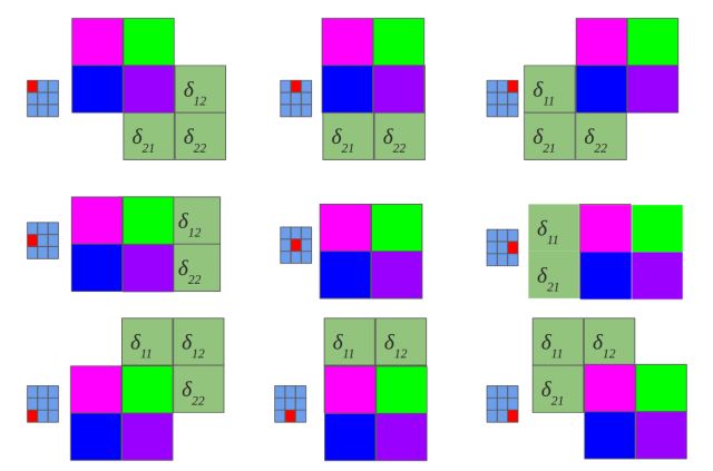
Section 1: valid convolution (input, kernel)

Section 2: gradient w.r.t. input of valid convolution (input, kernel) = weighted contribution of each input location w.r.t. gradient of Output

Section 3: full convolution(180 degree rotated filter, output)

As you can see, the calculation for the first three elements in section 2 is the same as the first three figures in section 3.
Hope this helps!
Convolutional Neural Networks backpropagation: from intuition to derivation
(部分latex公式无法显示,请查看原文链接『需FQ』)
Disclaimer: It is assumed that the reader is familiar with terms such as Multilayer Perceptron, delta errors or backpropagation. If not, it is recommended to read for example a chapter 2 of free online book ‘Neural Networks and Deep Learning’ byMichael Nielsen.
Convolutional Neural Networks (CNN) are now a standard way of image classification – there are publicly accessible deep learning frameworks, trained models and services. It’s more time consuming to install stuff like caffe than to perform state-of-the-art object classification or detection. We also have many methods of getting knowledge -there is a large number of deep learning courses/MOOCs, free e-books or even direct ways of accessing to the strongest Deep/Machine Learning minds such as Yoshua Bengio, Andrew NG or Yann Lecun by Quora, Facebook or G+.
Nevertheless, when I wanted to get deeper insight in CNN, I could not find a “CNN backpropagation for dummies”. Notoriously I met with statements like: “If you understand backpropagation in standard neural networks, there should not be a problem with understanding it in CNN” or “All things are nearly the same, except matrix multiplications are replaced by convolutions”. And of course I saw tons of ready equations.
It was a little consoling, when I found out that I am not alone, for example: Hello, when computing the gradients CNN, the weights need to be rotated, Why ?

The answer on above question, that concerns the need of rotation on weights in gradient computing, will be a result of this long post.
We start from multilayer perceptron and counting delta errors on fingers:
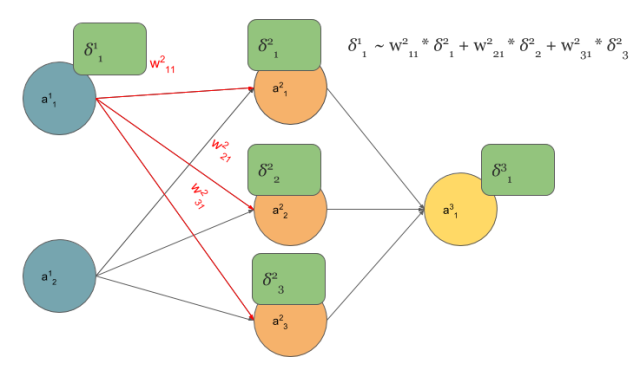
We see on above picture that 
But how do we connect concept of MLP with Convolutional Neural Network? Let’s play with MLP:
 Transforming Multilayer Perceptron to Convolutional Neural Network
If you are not sure that after connections cutting and weights sharing we get one layer Convolutional Neural Network, I hope that below picture will convince you:

Feedforward in CNN is identical with convolution operation
The idea behind this figure is to show, that such neural network configuration is identical with a 2D convolution operation and weights are just filters (also called kernels, convolution matrices, or masks).
Now we can come back to gradient computing by counting on fingers, but from now we will be only focused on CNN. Let’s begin:

Backpropagation also results with convolution
No magic here, we have just summed in “blue layer” scaled by weights gradients from “orange” layer. Same process as in MLP’s backpropagation. However, in the standard approach we talk about dot products and here we have … yup, again convolution:

Yeah, it is a bit different convolution than in previous (forward) case. There we did so called valid convolution, while here we do a full convolution (more about nomenclaturehere). What is more, we rotate our kernel by 180 degrees. But still, we are talking about convolution!
Now, I have some good news and some bad news:
- you see (BTW, sorry for pictures aesthetics :) ), that matrix dot products are replaced by convolution operations both in feed forward and backpropagation.
- you know that seeing something and understanding something … yup, we are going now to get our hands dirty and prove above statement <fn> before getting next, I recommend to read, mentioned already in the disclaimer, chapter 2 of M. Nielsen book. I tried to make all quantities to be consistent with work of Michael.
In the standard MLP, we can define an error of neuron j as:

where 

and for clarity, ")

But here, we do not have MLP but CNN and matrix multiplications are replaced by convolutions as we discussed before. So instead of 

 + b_{x,y}^{l+1} = sum limits_{a} sum limits_{b} w_{a,b}^{l+1}sigma(z_{x-a,y-b}^l)+ b_{x,y}^{l+1}")
Above equation is just a convolution operation during feedforward phase illustrated in the above picture titled ‘Feedforward in CNN is identical with convolution operation’
Now we can get to the point and answer the question Hello, when computing the gradients CNN, the weights need to be rotated, Why ?
We start from statement:

We know that 

 + b_{x',y'}^{l+1})}{partial z_{x,y}^l}")
First term is replaced by definition of error, while second has become large because we put it here expression on 

 + b_{x',y'}^{l+1})}{partial z_{x,y}^l} = sum limits_{x'} sum limits_{y'} delta_{x',y'}^{l+1} w_{a,b}^{l+1} sigma'(z_{x,y}^l)")
If 

 =sum limits_{x'}sum limits_{y'} delta_{x',y'}^{l+1} w_{x'-x,y'-y}^{l+1} sigma'(z_{x,y}^l)")
OK, our last equation is just …
= delta_{x,y}^{l+1} * w_{-x,-y}^{l+1} sigma'(z_{x,y}^l)")
Where is the rotation of weights? Actually  = w_{-x, -y}^{l+1}")
So the answer on question Hello, when computing the gradients CNN, the weights need to be rotated, Why ? is simple: the rotation of the weights just results from derivation of delta error in Convolution Neural Network.
OK, we are really close to the end. One more ingredient of backpropagation algorithm is update of weights 
 + b_{x,y}^l)}{partial w_{a,b}^l} =sum limits_{x}sum limits_{y} delta_{x,y}^l sigma(z_{x-a,y-b}^{l-1}) = delta_{a,b}^l * sigma(z_{-a,-b}^{l-1}) =delta_{a,b}^l * sigma(ROT180(z_{a,b}^{l-1}))")
So paraphrasing the backpropagation algorithm for CNN:
- Input x: set the corresponding activation
for the input layer.
- Feedforward: for each l = 2,3, …,L compute
and
- Output error
: Compute the vector
- Backpropagate the error: For each l=L-1,L-2,…,2 compute
- Output: The gradient of the cost function is given by
")
")
 sigma'(z_{x,y}^l)")
)")
The end