The improved Quicksort method of the present invention utilizes two pointers initialized at opposite ends of the array or partition to be sorted and an initial partition value Pvalue located at the center of the array or partition. The value at each of the end pointers is then compared to Pvalue. Sorting is accomplished by recursing the partition process for the two array segments bounded on one side by the final P valve location. This method prevents excessive recursions, and allows the identical array case to recurse to the ideal minimum: Log2(N). Also, by relaxing the offsider criteria to include elements equal to Pvalue, the present invention presents arrays of two valves or a very small range of valves from recursing excessively. Further, the sorting method of the present invention may test the final position of the initial Pvalue to determine whether it is in the center (75%-95%) portion of the array or subarray being positioned. If it is not, the first Pvalue is disregarded, and a new initial Pvalue is selected, preferably randomly selected from the larger subarray bounded on one side by the final Pvalue location resulting from the initial attempt. This method prevents arrays situated in "pipe organ" sequence from recursing excessively. In addition, a maximum recursion depth limit may be specified to force section of a new initial Pvalue if a recursion level exceeds the depth limit.
FIELD OF THE INVENTION
This invention relates to methods for sorting digitally stored information, and, in particular, to methods in accordance with the quicksort sorting method.
BACKGROUND OF THE INVENTION
Sorting is one of the most frequently conducted functions in data processing. Accordingly, providing sorting methods that work faster and with greater reliability are very important. These considerations are particularly important when sorting an array which is too large to be stored in a computer's random access memory.
Most programmers utilize the generic sorting utility supplied as part of their compiler library. For the C compiler, this is usually "Qsort." Virtually all C compiler Qsorts are direct descendants of the original AT&T UNIX system version written at Bell Labs circa 1978. This "Qsort" is very closely related to QuickerSort (ACM algorithm number 271) and not it's namesake, Qsort (ACM algorithm number 402).
The generic Qsort method is also related to the familiar binary search where each recursion halves the scope of the search. This relationship is most visible in the primary component of Qsort--the partition algorithm. It's job is to split a given array into exactly two pieces. To do this, it arbitrarily chooses an element as the partition value (Pvalue) and then considers the array from both ends to (ideally) the middle. Partition() looks for elements less than Pvalue on the high side and elements greater than Pvalue on the low side. When it has one of each, it swaps them and continues bringing the twin array indexes together. Where the indexes meet is where the Pvalue belongs, +/- one. After a final swap including Pvalue, Partition() is done. The partition(ed) array has three very important properties:
1) Pvalue is in it's FINAL position and can be further ignored.
2) All remaining elements are on their proper side or equal to Pvalue.
3) Partition can be called to further operate on either sub-array.
C.A.R. Hoare published the original "divide and conquer" "QuickSort" in July of 1961 as ACM algorithm number 64. This is the accepted root of any "Qsort," and is where the partition and recurse concept originated. Hoare selected his partition value randomly at all times. As discussed below, this penalizes the user when the array begins nearly sorted. In particular, Hoare scanned his arrays with a pointer starting from one end and continuing until an out of place value was found. After the first offsider was found, another pointer was scanned in from the opposite end until an offsider, or the first pointer, was hit. This scanning method is fraught with danger.
R. S. Scowen published his modification to the original algorithm and called it "QuickerSort" in November of 1965 as ACM#271. Scowen selected his partition value at the center of the sub-array. This is ideal for nearly sorted arrays and reverse sorted arrays but less than desirable for merging equal-length sorted blocks. Scowen also optimized the partition routine for the special case of two elements. Last, but not least, Scowen reduced the maximum depth of the stack by recursing into to the smaller partition first. Since the process was totally predictable, the "pipe organ" case (described further below) was reverse engineered to consistently present the worst possible partition value in the center. QuickerSort is also susceptible to the identical and 1's and 0's problems (described further below).
There was one other major attempt at modifying QuickSort by van Emden, M. H. in "Increasing the Efficiency of Quicksort," Communications of the ACM, Vol. 13, No. 9 (Sept. 1970). This article explains the mean partition value concept where the average value of the array is used for partitioning. It is believed that drawbacks of this approach include records that do not hash down to a neat value and the fact that an array element cannot be removed from consideration at each recursion level. The improvements alleged have not been reproducible and probably triggered the benchmark series by Rudolph Loeser in March of 1974.
The article "Implementing Quicksort Programs," Sedgewick, Robert, Communications of the ACM, Vol. 21, No. 10 (October 1978), concerns itself with machine efficiency rather than algorithm efficiency. It does note that "One can always `work backwards` to find a file which will require time proportional to N^2 to sort."
Sibley, Edgar H., "A Class of Sorting Algorithms Based on Quicksort," Communications of the ACM, Vol. 28, No.4 (April 1985), modifies Qsort to do a single partition. After each swap, the outermost parts of the array are bubble sorted to ensure that they remain in order until the indexes meet. It is believed that this method is inefficient because it does not partition efficiently, and this reference pertains more to bubble sorts than quickersorts.
Baer, Jean-Loup, "Improving Quicksort Performance with a Codeword Data Structure," IEEE Transactions on Software Engineering, Vol. 15 No. 5 (May 1989), concentrates on hashing records down to keys that can be sorted in memory. Conceptually, this is a case of sorting an index rather than a full record array. Each key can constitute a higher level --multi-record--view. Once the author explains his codeword key hash method, the article reverts to a very in-depth look at mechanical optimization techniques.
The shortcoming of past Qsort methods stems from the realization that all of Qsort's benefits accrue from partitioning the array as evenly as possible. Anytime the partition attempts consistently to converge away from the center of the array by a considerable margin, the Qsort will be less efficient. Therefore, a primary concern of the present invention is to maintain partition balance. Further investigation into MS-Qsort (and other implementations) reveals that the twin indexes are not brought together in lock-step. In other words, a single index is sequenced until it locates an offsider before the other index is even considered. This is the QuickerSort methodology. These shortcomings are particularly noticeable when an array happens to consist of identical elements. The twins meet each other at one end or the other and the array is partitioned into two subarrays, one of which is only one entry smaller than the original. Thus, this condition recurses N/2-2 times rather than the Log2(N) times QuickerSort is theoretically capable of achieving.
Most known Qsorts suffer from performance degradation under three conditions: (1) when all array elements are the same or; (2) when all array elements are of only two values (e.g. 1's and 0's); and (3) "pipe organ" inputs like 12344321. The pipe organ array breaks down because neither the first, last or center elements are an adequate choice for Pvalue. Although similar in effect to that of the identical elements condition, the pipe organ case requires a totally different sorting strategy. Most, if not all, commercial Qsorts are vulnerable to the pipe organ situation.
OBJECTS OF THE INVENTION
Accordingly, an object of the invention is to provide a Quicksort method that operates efficiently on a variety of types of arrays, including random, sorted, nearly sorted, reverse sorted, those containing many identical values or only a small range of values, and organ pipe organ situated data.
BRIEF DESCRIPTION OF THE DRAWINGS
FIG. 1 is a flow chart showing the method for calling the recursive Q sort method according to the present invention.
FIG. 2 is a flow chart showing one embodiment of the Q sort method according to the present invention.
FIG. 3 is a flow chart of the partitioning method of step 1.3.2 of FIG. 2.
SUMMARY OF THE INVENTION
The improved Quicksort method of the present invention utilizes two pointers initialized at opposite ends of the array or partition to be sorted. After each comparison, each pointer is synchronously moved toward each other if the compared elements are both on the proper side of the Pvalue. If only one element is on the proper side of the Pvalue, then the values are not swapped, but the movement of the pointer to the element on the opposite side of the Pvalue is suspended. The pointer to the element on the correct side of Pvalue continues to move toward the opposite pointer until it too encounters an element on the incorrect side of, or equal to, the Pvalue. At this point, the two elements are swapped. The comparison (and movement of both pointers) then resumes as discussed above until the pointers converge. The Pvalue is then relocated to this point to conclude the partition process. Sorting is accomplished by recursing this partition process for the two array segments bounded on one side by the final Pvalue location. This method prevents excessive recursions, and allows the identical array case to recurse to the ideal minimum: Log2(N). Also, by relaxing the offsider criteria to include elements equal to Pvalue, the present invention prevents arrays of two values or a very small range of values from recursing excessively. Further, the sorting method of the present invention may test the final position of the initial Pvalue to determine whether it is in the center (75%-95%) portion of the array or subarray being partitioned. If it is not, the first Pvalue is disregarded, and a new initial Pvalue is selected, preferably randomly selected from the larger subarray bounded on one side by the discarded Pvalue location resulting from the initial attempt. This method prevents arrays situated in a "pipe organ" sequence from recursing excessively. In addition, a maximum recursion depth limit may be specified to force selection of a new initial Pvalue if a recursion level exceeds the depth limit.
DETAILED DESCRIPTION
The improved Quicksort method of the present invention utilizes two pointers initialized at opposite ends of the array or partition to be sorted. After each comparison, each pointer is synchronously moved toward each other if the compared elements are both on the proper side of the Pvalue. If only one element is on the proper side of the Pvalue, then the values are not swapped, but the movement of the pointer to the element on the opposite side of the Pvalue is suspended. The pointer to the element on the correct side of Pvalue continues to move toward the opposite pointer until it too encounters an element on the incorrect side of, or equal to, the Pvalue. At this point, the two elements are swapped. The comparison (and movement of both pointers) then resumes as discussed above until the pointers converge. The Pvalue is then relocated to this point to conclude the partition process. Sorting is accomplished by recursing this partition process for the two array segments bounded on one side by the final Pvalue location. This method prevents excessive recursions by increasing the likelihood that it will converge in the middle, and allows the identical array case to recurse to the ideal minimum: Log2(N). Further, for each partition, the sorting method of the present invention may test the final position of the initial Pvalue to determine whether it is in the center (75%-95%) portion of the array or subarray being sorted. If it is not, the first Pvalue is disregarded, and a new initial Pvalue is selected, preferably randomly selected from the larger subarray bounded on one side by the Pvalue location resulting from the initial attempt. This method prevents arrays situated in "pipe organ" sequence from recursing excessively. In addition, a maximum recursion depth limit may be specified to abandon the current process and to start over with a more cautious configuration where the following attempt is significantly less likely to recurse as deep since the array has already been partially sorted and because of the increased caution.
This solution solves the problem where the array is filled with identical values and where the array is filled with a small number of unique values (e.g. 0,1). Note that the out-of-place criteria excludes the equal case initially but relaxes to include it after the first out-of-place member of a swappable pair has been located. This might seem to unnecessarily increase the number of swaps, but it also increases the likelihood that the partitioning concludes near the middle of the array. Testing shows the 0's & 1's case now typically recursing to 1.3 Log2(N), as shown below.
The following test results show results on three classes of arrays: random, 1's & 0's, and identical. The following tests were averaged from 21 trials, specifically N=100, 141, 200, 316, 500, 707, 1000, 1414, 2000, 3162, 5000, 7071, 10000, 14140, 20000, 31620, 50000, 70710, 100000, 141400, 200000.

The identical case proves that the ideal recursion is attainable, as long as no swapping is required. The 1's & 0's case has excellent performance, and averages only 25% more difficultly recursing than the ideal minimum. The random case averages 138% more difficult than the ideal minimum, but never exceeds 180% (2.8 * ideal) in this small sample. Note that the ratio of actual comparisons to the "ideal" N * Log2(N), the test beats the given ideal in both the identical and the 1's and 0's case.
N * Log2(N) does not consider the removal of partition values from the sorting process. There are 2 (depth) partition values per recursion level, with each Pvalue corresponding to a sub-array and call to partition(). But the critical fact is that none of these arrays include the Pvalues from the previous levels. Thus, each recursion cuts the array by more than half. Specifically (N-1)/2; where N is the size of the array to partition. For example, the first level has N elements, the second level has (2*(N-1))/2 elements, the third (4*((N-1)/2)-1)/2. Picture this as placing more and more ignorable spaces in the original array space:

A 40 element array can be reduced to 16 smaller 1 or 2 element arrays with only 4 recursions. Although one could continue to use Qsort all the way down to 2 elements, in one embodiment of the present invention, the method sorts two and three element arrays in special routines designed to take maximum advantage of the array in buffer situation. As shown below, 36% to 50% of the calls to the present invention's Qsort partition are directed to these two special routines.
A review of the number of comparisons needed to partition all the arrays at a given depth level reveals that the first level has N-1 mandatory comparisons. The second level lost one element and needs ((N-1)/2)-1 per sub-array, or N-3 total. This can also be stated as N minus the number of P's & Spaces on a level in the above diagram. The sequence is: 1, 3, 7 . . . (2 (depth+1)-1). Therefore, the total number of comparisons can be expressed as: ##EQU1##

Noting that the ideal level count is equal to both max__depth+1 and Log2(N), therefore, D can be replaced by with Log2(N)-1:
comps=(N+1) * Log2(N)-(2 (Log2(N)+1)-2)
Note that 2 (Log2(N)+1) can be further reduced to N * 2. Collecting terms and reducing, the result is:
comps=(N+1)*Log2(N)-(N-1)*2.
As N gets large; (N+1) and (N-1) converge to simply N. Thus, the equation above converges to:
comps=N*(Log2(N)-2)OR N* Log2(N/4)
As is evident from the identical case study above, this is approximately 83% of the classic N Log2(N) for a range.
Additional tests used the 21 different arrays sized from 100 to 200,000 elements, but the arrays were initialized with random data limited to a specific modulus. These tests expanded the 1's & 0's concept to research how the amount of work undertaken relates to the baseline ideals. These tests assume that the improved method of the present invention must expend a basic amount of energy just to consider the array (the ideal minimum) and anything over that is a function of the quantity of unique elements and their randomness. Since it's extremely difficult to judge "randomness", the following study only varies the uniqueness; on array initialization, elem=rand() % Modulus.

These ratios are well-behaved both from a Standard Deviation perspective and a trend basis. Note how slow baseline ideals grow in relation to element uniqueness. When the standard deviation is expressed as a percent, it remains fairly constant at 10.8% of recursions and 6.5% of comparisons. This suggests the following predicted averages:
Avg__recurs=Baseline__Ideal * (1+Ln(Modulus)/6.062)
Avg__comps=Baseline__Ideal * (1+Ln(Modulus)/23.04)
Another embodiment of the present invention helps to solve arrays sorted in "pipe organ" fashion, such as "12344321." This embodiment involves arbitrarily creating a target area or "sweet-spot" in the center of the array. If a partition converges in the sweet-spot then nothing changes from before. But if not, the array is repartitioned with a new partition value based on what is learned from the first attempt. In one embodiment, the second partition is final. One object of this embodiment is to maintain partition balance. Bad partitions will always leave a large majority of the array on one side. In such instances, one of the only facts known about the partitioned array is that all of the elements on the small side are just as bad or worse than the initial Pvalue. Therefore, the next partition value is selected from the bigger side.
However, the size of the "sweet spot" is an important factor. Empirical research reveals that correct selection of a sweet spot brings the pipe-organ case down to a very reasonable 1.82 times the baseline comparisons ideal. Recursions are very reasonable too, seldom more than 2 times baseline.

Good results were also achieved for randomly sorted arrays, as shown by the following table averaging several tests of the specified array size for sweet spots of 75%, 87.5%, and 93.75%. These sweet spot sizes imply that arrays must be a minimum size before the non-sweet spots are at least an element wide. {This minimum is in braces} All the numbers in the following table are the comparisons ratio to ideal followed by the standard deviation therewith, as a percent, in parenthesis:
Sorts of 30 Bit RANDOM number arrays with various size sweet spots

The above shows that randomized arrays require 1.39 times the baseline ideal amount of comparisons without repartitioning. When a 75 % sweet spot is used, randomized arrays require 6.07% more comparisons than before but only grow to 1.82 times the baseline for the pipe organ, showing an improvement over using no sweet spot. An 87.5% sweet spot implies 2.45% and 1.91 times the baseline, respectively. This shows that by selecting different sweet spots, pipe organ stability is traded off for an increased amount of comparisons on the typical random case. As noted above, a pipe organ tries to recurse to N/2-2 without sweet spot repartitioning. A slightly different way to view this is as wasting the difference between N/2-2 and the archetypical 2.4 * Log2(N/4) for a fully random order:

The above table suggests that 6.8 recursion levels can be incurred before policing the partition balance with a 93.75% sweet spot size. As noted above, this translates to an increase in comparisons of only 1.35% over doing no repartitioning at all. As the pipe organ cases discussed below confirm, the method of one embodiment of the present invention can recurse up to four times the baseline minimum in a worst case scenario, even though the (much more common) random case only recurses 2.4 times the baseline. Nevertheless, Log2(N) performance is achieved. Applications that need to sort more than a hundred million elements should limit the recursion depth by using the 87.5% sweet spot, as it's worst case limit is 2.5 billion elements.
In another embodiment of the present invention, the method will "gracefully" stop recursing once it reaches a preset RECURSION__LIMIT value. After it backs out of the sort in progress without corrupting anything, it simply re-starts the sort with the sweet spot reduced to 75%. It is practically guaranteed not to recurse as deep since the file was partially sorted on the first attempt. However, this feature should not ordinarily be implemented to routinely stretch the practical working limit of one billion elements except in a pure pipe organ situation.
In summary, a 93.75% sweet spot implies that the repartitioning test cannot fail for subarrays of less than 32 elements. Although pipe organ arrays can run poorly up to that point, they will be sternly repartitioned thereafter. As the following table shows, all ratios seem to stabilize by the time the organ gets up to 64 elements in size. After that, they average 1.93 times the baseline comparisons and 2.77 times the baseline recursions. This stability comes at a price though, as a random array comparison performance rises from 1.39 to 1.41 times the baseline. A summary of the pipe organ's performance is as follows:


Where:
N is the elemental size of the array.
Cnt is the number of trial runs in line averages.
Comps is the ratio of Comparisons to ideal: N * Log2(N/4). {The next four columns are expressed as a percent of N}
Part__3 +is the number of calls to partition for sub-arrays>3 elem.
Re-Part is the number of re-partitions due to missed sweet-spots.
Part__3 is the number of calls to partition/sort 3 elem sub-arrays.
Part__2 is the number of calls to partition/sort 2 elem sub__arrays.
Rec is the average recursion depth for the given array size.
Ratio__I is the recursion depth relative to ideal: floor(Log2(N/4)).
Time is the sorting time divided by actual comparisons; MicroSeconds.
In analyzing the above results, it is important to keep in mind that they are based on the most difficult array type for aquicksort to handle. Note that the 93.75% sweet spot allows recursions to grow as N/2-2 up to the 32 element police kick-in point. Sometimes, the optimized twosort() and threesort() saves a recursion. Nevertheless all the ratios are relatively stable when 64 or more elements are sorted. Each ratio parameter is discussed individually after the next table.
The sorting method of the present invention expends a baseline amount of energy just to consider a given array. Ideally, if the array is already in order, this is the only energy expended. If only a small percentage of the elements are out of order, the energy rises a small percentage. It is interesting to note how the initial order affects the energy. Reverse sorted arrays require only the baseline amount of comparisons. 30 bit random number arrays require 1.4 times the baseline minimum comparisons. Sorting pipe organ ordered arrays can require up to 2.1 times the baseline comparisons. This demonstrates that the pipe organ case is very nearly the worst possible order for a Quicksort method, and fortunately occurs somewhat rarely in real life. It is possible to use the pipe organ case to predict a worst case rise above baseline within a three sigma (99.865%) confidence interval as follows.
Max Comparisons=2.13 * Baseline, Max Recursions=4.5 * Baseline
Typ Comparisons=1.41 * Baseline, Typ Recursions=2.40 * Baseline
Min Comparisons=1.00 * Baseline, Min Recursions=1.00 * Baseline
Comps. Baseline=N * Log2(N/4), Recur Baseline=floor(Log2(N/4))
The random performance is shown below.

(The parameters have exactly the same meaning as they did above.)
It is first worth noting that the maximum depth reached past 50 recursions for the largest array of 33,554,432 elements and, that the average recursion of 2.4 times the ideal. Assuming an absolute worst case ratio of 4, up to 92 recursions could occur for the largest array above. Nevertheless, a 100 recursion limit should perform adequately for any situation.
In addition to the number of comparisons and recursions, another factor of interest is the number of times that partition(), threesort(), & twosort() are called. The number of calls thereto can be neatly expressed as a percentage of N. Ideally, partition() would be called 25%N times and split another 25%N between twosort() and threesort(). It's notable here, that partition() is being called at 39.8%N and 20.1%N is going nearly equally between twosort() and threesort(). The latter two routines being optimized partition/sort methods for the smallest sub-arrays of length two and three, respectively. Also, note that repartitioning occurs only 0.44%N times. Compared to the 39.8%N calls it is evident that repartitioning 1.1% of the sub-arrays occurs for sub-arrays greater than 3 elements in size. But, this can rise to 1.96/39.98 or 4.9% to control the pipe organ case. Accordingly, repartitioning does not help efficiency in the random case, but merely guarantees stability.
Although several authors postulate that the traditional quicksort is inefficient for "small" arrays of 9 elements or less (e.g., "Implementing Quicksort Programs by Robert Sedgewick of Brown University), the quicksort method of the present invention does not demonstrate such shortcomings except those accumulated from calculating the median index value (the sweet spot test may be skipped for n<32) and not taking advantage of the sub-array in buffer condition. Inefficiencies of prior quicksort methods likely accrue from not dropping the partition value from consideration on recursions. Because 1/3 to 1/2 of the total recursive calls are sub-arrays where n<4, optimization efforts are worth the extra effort.
Although the above discussion focuses on the number of comparisons and recursion levels, the issue of sorting time is also worth discussing. The above tests tracked the number of seconds required to perform the sort, not including the time required to initialize the array or verify sort correctness. Knowing that 90% or more of the time is spent loading and comparing records, the total time can be divided by the actual number of comparisons made. This microsecond value is displayed in the rightmost column of the above study and is a composite of three 286-class machines working full time on a LAN. The last value in said column was made using a 50 Mhz 486 to speed up the heavy end of the study. Regardless, the way to predict the sorting time is to perform a small sort of say, 32768 elements and note the time; 212.8 micro-seconds in this case. Then, calculate any time estimate from 212.8E-6 * 1.4 * N * Log2(N/4).
In summary, the basic Qsort can be stabilized by relaxing the offsider criteria and allowing partition() a second chance when it misses the sweet spot. The worst case "pipe organ" scenario succumbs to 1.9 times ideal, up only slightly from 1.4 times ideal for the completely random case.
To provide another benchmark between the method of the present invention and those of the prior art, it is noted that Rudolph Loeser, in "Some Performance Tests of QuickSort and Descendants," Communications of the ACM, Vol. 17, No. 3 (March 1974), published benchmark tests for his quicksort method. These results derived that the optimum number of comparisons is N*Log2(N) (although the above results derived that the optimum number of comparisons is N*Log2(N/4) for the present invention). Accordingly, a set of benchmark results of present method against those published by Loeser, for various types of array sorts is shown below. Table I is for the present invention (called WdaSort) configured with a 93.75% sweet spot. The columns are:
N--The size of the array being sorted.
M--The number of array elements out of place in almost sorted order, and the number of equal-length blocks in the merge blocks order.
Cnt--The number of WdaTest2 program runs underlying the line averages.
Comps__W--The ratio of the number of comparisons to the ideal calculated by the inventor: N * Log2(N/4). This value has been included for discussion purposes in lieu of the Loeser ratio because it is very stable among initial (pre-sort) orders.
Sd--The standard deviation of the column immediately to the left of the value, expressed as a percent. This parameter is calculated for several columns.
Comps__L--The ratio of the number of comparisons to N * Log2(N). This ratio is sometimes expressed as the asymptotic limit when N→ω, but it has been shown that N * Log2(N/4) converges faster.
Fetch__L--The ratio of the number of record fetches to N * Log2(N). (Rudolph Loeser compares everything by this basis)
Save__L--The ratio of the number of record saves to N*Log2(N).
Part4+--The number of calls to initially partition sub-arrays of length four or greater, expressed as a percentage of N (rather than Loeser's ratio) so that some basic properties of WdaSort are more apparent. This has no direct correlation to Loeser's study.
RePart--The number of times that the initial partitions had to be re-done because they balanced outside of the sweet spot. Although this is also a call to partition a sub-array of length four or greater, it is counted independently of the preceding column. It is expressed as a percentage of N.
Sort3--The number of calls to sort out a three element sub-array, expressed as a percent of N.
Sort2--The number of calls to sort out a two element sub-array, expressed as a percent of N.
Rec--The maximum number of recursive WdaSort calls.
Ratio__W--The ratio of the recursive calls to the ideal calculated by Wda: Log2(N/4). This value has been included for discussion purposes in lieu of the Loeser ratio because it is very stable among initial (pre-sort) orders. Loeser's recursion ratio can not be directly compared because it is based on N*Log2(N).
Time--This value was obtained by dividing the total sorting time by the number of comparisons made. It is expressed in Micro-Seconds and represents the time required for a 386/25 PC to load a record over the LAN and compare it to the partition element. The consistency of this value demonstrates the real time predictability of WdaSort as a function: Total--Time=Time * Comps__W * N * Log2(N/4).
All sorting algorithms are affected by the array's initial order. Loeser benchmarked with five different cases; Already Sorted, Sorted in Reverse order, Random order, Almost sorted order, and equal-length (or merge) block order.


If the array is already sorted, notice that WdaSort has Comps__W at the ideal; 1.000. The reason that the smaller arrays are not displayed as exactly 1.000 arises from the ideal comps equation: (N+1)*Log2(N)-(N-1)*2. As N gets larger, (N+1) and (N-1) converge to simply N and the equation can be more neatly expressed as N*Log2(N/4). But, even with the smallest 32 element array, the inaccuracy introduced here is only 7.3%.
Comparing WdaSort's Comps__L column to Loeser's "Compares" column shows that Wda Sort beats all Qsort derivatives and almost exactly matches the shellsort comparisons. Although StringSort is almost twice as fast as WdaSort in this nothing-to-do situation, StringSort demonstrates very poor performance when real work arises as clearly demonstrated in the almost sorted case.
It is interesting to note that the Fetch__L column is nearly equal to the Comps__L column. The difference comes from loading the initial partitioning element. The difference quickly becomes negligible as the size of the array increases.
The Save__L column is zero for the already sorted order and never goes higher than 0.456. Comparing it to Loeser's "Stores" indicates that WdaSort is among, if not the, fastest.
Part4+ is called exactly 25% of N times. Also, note that Sort3 plus Sort2 is exactly 25% of N again. These are the hypothetical minimums. Of course there was no re-partitioning to do either.
Ratio__W confirms the ideal recursion formula: Log2(N/4).
Time tells us that the largest 33,554,432 element sort took 15 hours to perform.
The Reverse Sorted Order
WdaSort performs this case almost exactly the same as the Already Sorted case, above. The only exception being Save--L. Comparing this with Loeser's "Stores" shows that QuickSort and Qsort match WdaSort, but nobody beats it. Here, the efficiency of quicksort methods are apparent when there is real work to do.
Few of the algorithms handled the simple reversing of order efficiently.
The Random Order
This is the case traditionally considered the most common burden for a sort method. Few things alter the difficulty of a randomized array except when the number of array elements approach the numeric range of one of the elements. This is pertinent for purposes of comparison because Loeser apparently filled his test arrays with 15 to 16 bit random numbers. This indicates that there will probably be several duplicate values in his largest arrays, thereby reducing the complexity of the sort. The above tests use 30 random numbers and could raise WdeSort's ratio's ever so slightly in comparison.
Not that Comps__W hovers around 1.41 with a standard deviation of about 1.5% for this case. Perfecting this value was achieved in a trade off between 1.39 with no safety measures and 1.47 for the best behaved sort, from a maximum recursion depth point of view, using a 75% sweet spot.
Comps__L almost exactly mirrored that of QuickerSort. Save__L almost exactly mirrored that of QuickSort.
Note that Part4+ is called just under 40% N times and RePartitions were only done 0.44% N times or for 1.11% of the Part4+ calls. Also, Sort3 and Sort2 are being called at just over 10% N times each. The number values behind these percentages are but a fraction of the number of fetch & compare iterations. Therefore, there is no linear component in the WdaSort time function: Time*Comps__W*N*Log2(N/4).
The Ratio__W value averages 2.4 with a standard deviation of 4.2%. Note that the maximum recursion depth reached just slightly past halfway up the 100 recursion limit for our largest array of 33,554,432 elements. Incidentally, the Time value implies that sorting this array took about 21 hours.
The Almost Sorted Order
This is one of the most common cases in practice--sort an array, append or update a few elements, and then re-sort the array. This is also where the present method clearly demonstrates its superiority for most all of the columns, even Fetch--L. Note that Comps__W rises somewhat proportionally to the percentage of out-of-place entries in the array. A first attempt to quantify Comps__W as a function of M/N resulted in 1.055+0.975*M/N.
Qsort performance degrades significantly in this case. Virtually all statistics are poor, especially the Standard Deviations.
The Merge (equal-length) Block Order
This is just about the worst case for the quicksort family. Merging two equal length blocks performs similar to the dreaded pipe organ case with Comps__W averaging about 1.95. But increasing the block count to four reduces it to a more reasonable 1.6.
Ratio__W shows it's worst case performance too, going as high as 4.4 for 2,097,152 & 2. If an application regularly needs to work on such arrays, reducing WdaSort's sweet spot to 75%N will bring Ratio__W down to a more reasonable 2.11 in exchange for increasing Comps__W by about five percent across the board.
Conclusion
It is interesting to note that Loeser did not benchmark any of the cases in which Qsort operates least effectively, namely, identical elements, 1's and 0's, and the pipe organ case. However, the method of the present invention has outperformed the Loeser benchmarks on all of the problem cases.
WdaSort is designed to be part of a programming library that can be called upon for small and large jobs alike. The calling interface makes no direct references to the array and only requires three routines: load a record, save a record, and compare two loaded records. This way, the programmer is free to store and manipulate the array elements as he or she so chooses.
WdaSort currently requires up to 3 Kb of free stack space under DOS to perform. This stack size should allow sorting arrays approaching a billion elements in size. If the size and/or complexity of an array exceeds this limit, the program gracefully backs out of the first sort attempt and reconfigures itself for an automatic, and more cautious, retry. Where, the second attempt is almost guaranteed to succeed since the file has already been partially sorted. This cautious configuration typically requires only half as much stack depth to sort complex arrays.
In one embodiment, a three record buffer is used in the Partition code. One element is loaded with the partition value (Pvalue). One element holds an array element being compared to the Pvalue, and one element holds the opposite value being compared to the Pvalue. That way, the Pvalue is loaded only once per call to partition, record swaps can be performed by merely cross saving the buffers. This permits quick processing even for large arrays of, for example, over one million elements, even if stored on a hard disk or other computer peripheral storage device.
The present invention also utilizes a programmer interface unlike any other commercially available known sort. The standard C library Qsort() is designed strictly for memory arrays. It is called with array pointer, number of elements, element size, and function to compare elements by address. The caller has no control of the array while it is being sorted, so everything is constrained by memory limitations. The WdaSort or the present invention, on the other hand, operates through a three element buffer and requests that the programmer place specific array elements (or records if you will) in one of the three buffers. This allows the most freedom for writing memory sorts, disk file sorts, or any cached mixture thereof. WdaSort is called with first and last array indexes, loadbuf function, savebuf function, and compare__buffer function. WdaTest2.c in the Appendix provides an example of how this is best used.
WdaSort may be offered as part of the standard `C` programming environment of any platform. WdaSort will be tremendously faster on the 32 bit machines since nearly all variables are in long integer format.
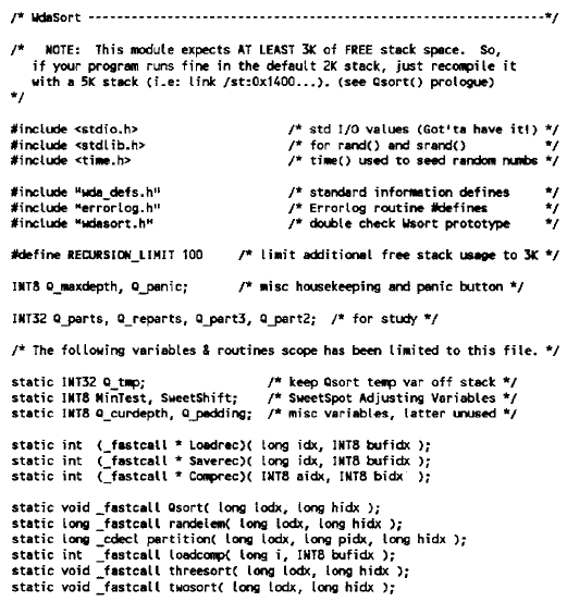
Source code for implementing the sorting method according to the present invention is shown in the appendix. ##SPC1##
|