仅仅为了学习Keras的使用,使用一个四层的全连接网络对MNIST数据集进行分类,网络模型各层结点数为:784: 256: 128 : 10;
使用整体数据集的75%作为训练集,25%作为测试集,最终在测试集上的正确率也就只能达到92%,太低了:
              precision    recall  f1-score   support

         0.0       0.95      0.96      0.96      1721
         1.0       0.95      0.97      0.96      1983
         2.0       0.91      0.90      0.91      1793
         3.0       0.91      0.88      0.89      1833
         4.0       0.92      0.93      0.92      1689
         5.0       0.87      0.86      0.87      1598
         6.0       0.92      0.95      0.94      1699
         7.0       0.94      0.93      0.93      1817
         8.0       0.89      0.87      0.88      1721
         9.0       0.89      0.90      0.89      1646

   micro avg       0.92      0.92      0.92     17500
   macro avg       0.91      0.92      0.91     17500
weighted avg       0.92      0.92      0.92     17500
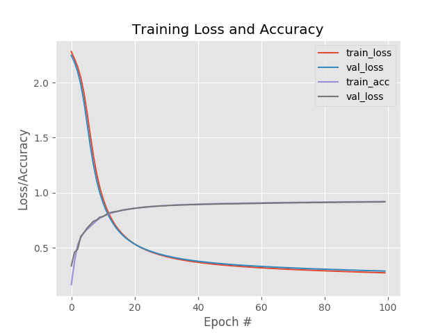
训练过程中,损失和正确率曲线:
上面使用的优化方法是SGD,下面在保持所有参数不变的情况下,使用RMSpro进行优化,最后的结果看起来好了不少啊达到98%:
              precision    recall  f1-score   support

         0.0       0.99      0.99      0.99      1719
         1.0       0.99      0.99      0.99      1997
         2.0       0.99      0.97      0.98      1785
         3.0       0.97      0.98      0.97      1746
         4.0       0.98      0.98      0.98      1654
         5.0       0.97      0.97      0.97      1556
         6.0       0.99      0.99      0.99      1740
         7.0       0.98      0.97      0.98      1845
         8.0       0.97      0.98      0.97      1669
         9.0       0.96      0.97      0.97      1789

   micro avg       0.98      0.98      0.98     17500
   macro avg       0.98      0.98      0.98     17500
weighted avg       0.98      0.98      0.98     17500

这相差有些大了啊,损失一开始就比较低,正确率就比较高;
在执行一些epoch之后,训练集损失降低到一定程度并趋于平缓,而测试集的损失却在逐渐升高,看来是过拟合了啊。
也就是说大概在最初几个epoch的时候训练集的损失比较低,而且测试集的损失达到最低,正确率也都不错;应该就可以停止了。
代码:
#!/usr/bin/env python
# -*- coding: utf-8 -*-
# @Time : 19-5-9

"""
implement simple neural networks using the Keras libary
"""

__author__ = 'Zhen Chen'


# import the necessary packages
from sklearn.preprocessing import LabelBinarizer
from sklearn.model_selection import train_test_split
from sklearn.metrics import classification_report
from keras.models import Sequential
from keras.layers.core import Dense
from keras.optimizers import SGD
from sklearn import datasets
import matplotlib.pyplot as plt
import numpy as np
import argparse

# construct the argument parse and parse the arguments
parser = argparse.ArgumentParser()
parser.add_argument("-o", "--output", default="./Training Loss and Accuracy.png",
                    help="path to the output loss/accuracy plot")
args = parser.parse_args()

# grab the MNIST datset (if this is your first time running this
# script, the download may take a minute -- the 55MB MNIST datset
# will be downloaded
print("[INFO] loading MNIST (full) dataset...")
dataset = datasets.fetch_mldata("MNIST Original")

# scale the raw pixel intensities to the range [0, 1.0], then
# construct the training and testing splits
data = dataset.data.astype("float") / 255.0
(trainX, testX, trainY, testY) = train_test_split(data, dataset.target, test_size=0.25)

# convert the labels form integers to vectors
lb = LabelBinarizer()
trainY = lb.fit_transform(trainY)
testY = lb.fit_transform(testY)

# define the 784-256-128-10 architecture using Keras
model = Sequential()
model.add(Dense(256, input_shape=(784,), activation="sigmoid"))
model.add(Dense(128, activation="sigmoid"))
model.add(Dense(10, activation="softmax"))

# train the model using SGD
print("[INFO] training network...")
sgd = SGD(0.01)
model.compile(loss="categorical_crossentropy", optimizer=sgd, metrics=["accuracy"])
H = model.fit(trainX, trainY, validation_data=(testX, testY), epochs=100, batch_size=128)

# evaluate the network
print("[INFO] evaluating network...")
predictions = model.predict(testX, batch_size=128)
print(classification_report(testY.argmax(axis=1),
                            predictions.argmax(axis=1),
                            target_names=[str(x) for x in lb.classes_]))

# plot the training loss and accuracy
plt.style.use("ggplot")
plt.figure()
plt.plot(np.arange(0, 100), H.history["loss"], label="train_loss")
plt.plot(np.arange(0, 100), H.history["val_loss"], label="val_loss")
plt.plot(np.arange(0, 100), H.history["acc"], label="train_acc")
plt.plot(np.arange(0, 100), H.history["val_acc"], label="val_loss")
plt.title("Training Loss and Accuracy")
plt.xlabel("Epoch #")
plt.ylabel("Loss/Accuracy")
plt.legend()
plt.savefig(args.output)