library(devtools)
install_github("jennybc/gapminder")
> library(gapminder)
> data(gapminder)
> head(gapminder)
country continent year lifeExp pop gdpPercap
1 Afghanistan Asia 1952 28.801 8425333 779.4453
2 Afghanistan Asia 1957 30.332 9240934 820.8530
3 Afghanistan Asia 1962 31.997 10267083 853.1007
4 Afghanistan Asia 1967 34.020 11537966 836.1971
5 Afghanistan Asia 1972 36.088 13079460 739.9811
6 Afghanistan Asia 1977 38.438 14880372 786.1134
> dat1952=gapminder[gapminder$year==1952,]
> x=dat1952$lifeExp
> mean(x<=40)
[1] 0.2887324
> mean(x<=40)
[1] 0.2887324
> mean(x<=60&x>=40)
[1] 0.471831
> mean(x<=60&x>=40)
[1] 0.471831
> mean(x<=60)-mean(x<=40)
[1] 0.4647887
> prop=function(q){
+ mean(x<=q)
+ }
> prop(40)
[1] 0.2887324
> qs=seq(from=min(x),to=max(x),length=20)
props=sapply(qs,prop)
plot(qs,prop)
props=sapply(qs,function(q)mean(x<=q))
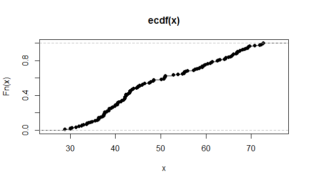
plot(ecdf(x))
> library(gapminder)
> data(gapminder)
> dat1952=gapminder[gapminder$year==1952,]
> y=dat1952$pop
> log10(y)
[1] 6.925587 6.108124 6.967526 6.626555 7.252294 6.939080 6.840594 5.080796 7.671051
[10] 6.941034 6.240128 6.459892 6.445760 5.645725 7.752836 6.861827 6.650305 6.388389
[19] 6.671528 6.699757 7.169838 6.111160 6.428534 6.804659 8.745281 7.091694 5.187340
[28] 7.149219 5.931908 5.966760 6.473782 6.589081 6.778715 6.960242 6.636889 4.800366
[37] 6.396434 6.550076 7.346809 6.310240 5.336388 6.157988 7.319334 6.611776 7.627977
[46] 5.623975 5.453807 7.839767 6.746712 6.888362 6.497811 6.425575 5.763917 6.505352
[55] 6.181115 6.327543 6.977906 5.170150 8.570543 7.914089 7.237343 6.735740 6.470139
[64] 6.209760 7.678209 6.154148 7.936810 5.783842 6.810504 6.947703 7.321134 5.204120
[73] 6.158220 5.874335 5.936166 6.008485 6.677873 6.465056 6.829199 6.584124 6.009687
[82] 5.713117 7.479205 5.903450 5.616826 6.997352 6.809312 7.303045 5.686485 6.962963
[91] 7.016281 6.299898 6.066620 6.528848 7.520078 6.522148 5.705721 7.616439 5.973165
[100] 6.191975 6.904483 7.350998 7.410449 6.930748 6.347720 5.411114 7.220892 6.403965
[109] 4.778231 6.602676 6.440214 6.836333 6.331073 6.051924 6.551223 6.173046 6.402604
[118] 7.154270 7.455604 6.902130 6.929657 5.462762 6.852765 6.682596 6.563665 6.931985
[127] 6.920276 7.328163 6.086044 5.821415 6.562023 7.347050 6.765281 7.702689 8.197427
[136] 6.352754 6.735564 7.419077 6.013084 6.695817 6.426836 6.488679
> sd(log10(y))
[1] 0.7070292
question: what is the difference between the sample standard deviation and the population standard deviation?
> sqrt(mean((log10(y)-mean(log10(y)))^2))
[1] 0.7045353
# the sample standard deviation
sd(logpop)
# the population standard deviation
sqrt(mean((logpop - mean(logpop))^2))
Standardize the log10 population size vector, by subtracting the mean and dividing by the standard deviation,as in: (a - b)/c
What is the z-score of the country with the largest population size? (you can use max(z) to see the very last and largest value).
z=(log10(y)-mean(log10(y)))/sd(log10(y))
max(z)

head(pnorm(log10(y),mean=mean(log10(y)),sd=sd(log10(y))))
mean(z)
sd(z)
head(pnorm(z))