dat = read.csv("femaleMiceWeights.csv")
mean(dat[13:24,2]) - mean(dat[1:12,2])
s = split(dat[,2], dat[,1])
stripchart(s, vertical=TRUE, col=1:2)
abline(h=sapply(s, mean), col=1:2)
abline(h=sapply(s, mean), col=1:2)

> sum(dat[13:24,2]<mean(dat[1:12,2]))
[1] 3
> sum(dat[1:12,2]>mean(dat[13:24,2]))
[1] 3
> highfat=s[["hf"]]
> highfat
[1] 25.71 26.37 22.80 25.34 24.97 28.14 29.58 30.92 34.02 21.90 31.53 20.73
> sample(highfat,6)
[1] 20.73 26.37 24.97 25.34 21.90 28.14
> sample(highfat,6,replace=TRUE)
[1] 21.90 29.58 24.97 22.80 21.90 28.14
> highfat>30
[1] FALSE FALSE FALSE FALSE FALSE FALSE FALSE TRUE TRUE FALSE TRUE FALSE
> as.numeric(highfat>30)
[1] 0 0 0 0 0 0 0 1 1 0 1 0
> sum(highfat>30)
[1] 3
> mean(highfat>30)
[1] 0.25
> population = read.csv("femaleControlsPopulation.csv")
> population = population[,1]
> mean(population)
[1] 23.89338
> sample(population,12)
[1] 22.87 19.96 24.46 21.58 28.43 21.77 24.55 26.07 22.99 24.96 20.69 29.99
> mean(sample(population,12))
[1] 23.33333
> sampleMean=replicate(10000,mean(sample(population,12)))
> head(sampleMean)
[1] 24.07167 22.85250 24.73583 22.95833 22.80750 25.97333
> plot(sampleMean)
> null=replicate(10000,mean(sample(population,12))-mean(sample(population,12)))
> head(null)
[1] 1.0425000 -1.9241667 -4.8841667 -1.6341667 -0.2450000 -0.5566667
> plot(null)

> hist(null)
> head(null)
[1] 1.0425000 -1.9241667 -4.8841667 -1.6341667 -0.2450000 -0.5566667
> plot(null)
> hist(null)
> diff=mean(dat[13:24,2])-mean(dat[1:12,2])
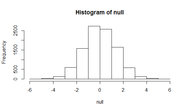
> mean(null>abs(diff))
[1] 0.0148
> mean(abs(null)>abs(diff))
[1] 0.0279