ENAS
2018-ICML-Efficient Neural Architecture Search via Parameter Sharing
来源:ChenBong 博客园
- Hieu Pham(Google Brain、CMU),Quoc V. Le(Google Brain),Jeff Dean(Google Brain)
- GitHub:
- https://github.com/carpedm20/ENAS-pytorch 2.2k
- https://github.com/melodyguan/enas 1.5k
- Citation:625
Introduction
We propose Efficient Neural Architecture Search (ENAS), a fast and inexpensive approach for automatic model design
提出了ENAS,一种快速且计算开销小的自动化模型设计方法。
In ENAS, a controller discovers neural network architectures by searching for an optimal subgraph within a large computational graph.
在ENAS中,控制器从一个大的计算图中,搜索最佳子图
On the CIFAR-10 dataset, ENAS finds a novel architecture that achieves 2.89% test error, which is on par with the 2.65% test error of NASNet.
在cifar10上 2.89% err,对比NASNet方法是2.65% err
On Penn Treebank, our method achieves a test perplexity of 55.8, which significantly outperforms NAS’s test perplexity of 62.4 (Zoph & Le, 2017) and which is a new state-of-the-art among Penn Treebank’s approaches that do not utilize post-training processing.
在Penn Treebank上,我们的方法的perplexity是55.8,远低于NAS方法的62.4,是新的sota
Importantly, in all of our experiments, for which we use a single Nvidia GTX 1080Ti GPU, the search for architectures takes less than 16 hours.
很重要的一点,我们的实验使用一张1080ti 跑了16小时即可
Due to its efficiency, we name our method Efficient Neural Architecture Search (ENAS).
由于高效性,因此叫做ENAS
Motivation
In NAS, an RNN controller is trained in a loop: the controller first samples a candidate architecture, i.e. a child model, and then trains it to convergence to measure its performance on the task of desire.
The controller then uses the performance as a guiding signal to find more promising architectures.
在NAS方法中,RNN控制器循环训练,1. sample 一个子网络,2. 训练子网络至收敛,获得子网络的性能指标(测试集精度)3. RNN控制器使用性能指标作为信号,生成更好的模型
We observe that the computational bottleneck of NAS is the training of each child model to convergence, only to measure its accuracy whilst throwing away all the trained weights.
我们认为,NAS计算开销大的主要原因在于,每个子网络都需要训练到收敛,但需要的只是子网络的acc,而把训练好的权重都丢弃。
Contribution
The main contribution of this work is to improve the efficiency of NAS by forcing all child models to share weights to eschew training each child model from scratch to convergence.
本文的主要贡献是,通过强制所有子网络贡献参数,而避免from scratch 训练每个子网络
Sharing parameters among child models allows ENAS to deliver strong empirical performances, while using much fewer GPUhours than existing automatic model design approaches, and notably, 1000x less expensive than standard Neural Architecture Search.
子模型间共享参数,可以让ENAS有很好的表现同时有着更少的GPU hours,比NAS方法少了1000倍。
Method
Central to the idea of ENAS is the observation that all of the graphs which NAS ends up iterating over can be viewed as sub-graphs of a larger graph.
ENAS的核心是,观察到NAS最终得到的图都可以看成大图的子图
In other words, we can represent NAS’s search space using a single directed acyclic graph (DAG).
就是说,我们可以用一个有向无环图(DAG)来表示NAS的搜索空间
Figure 2 illustrates a generic example DAG, where an architecture can be realized by taking a subgraph of the DAG.
图2是一个DAG,可以通过选取其中的子图来实现不同的cell结构

Intuitively, ENAS’s DAG is the superposition of all possible child models in a search space of NAS, where the nodes represent the local computations and the edges represent the flow of information.
ENAS的DAG是搜索空间中所有子模型的叠加,节点代表计算操作,边代表信息流动
The local computations at each node have their own parameters, which are used only when the particular computation is activated.
每个节点上的操作都有自己的参数,尽在当前节点激活时才使用
Therefore, ENAS’s design allows parameters to be shared among all child models,
因此,ENAS允许不同子模型之间共享参数
In the following, we facilitate the discussion of ENAS with an example that illustrates how to design a cell for recurrent neural networks from a specified DAG and a controller (Section 2.1).
下面通过一个示例来说明如何从一个DAG中设计cell
We will then explain how to train ENAS and how to derive architectures from ENAS’s controller (Section 2.2).
我们将介绍如何训练ENAS以及如何从控制器RNN中导出cell结构(section 2.2)
Finally, we will explain our search space for designing convolutional architectures (Sections 2.3 and 2.4).
最后我们将说明我设计卷积网络的搜索空间
Sec 2.3. Designing Convolutional Networks
Recall that in the search space of the recurrent cell, the controller RNN samples two decisions at each decision block:
what previous node to connect to and
what activation function to use.
RNN cell的搜索空间中,控制器RNN在每个block进行2个预测:
1)连接到之前哪个节点
2)使用哪种激活函数
In the search space for convolutional models, the controller RNN also samples two sets of decisions at each decision block:
what previous nodes to connect to and
what computation operation to use.
在卷积模型的搜索空间中,控制器RNN也在每个block进行2个预测:
1)连接到之前哪个层
2)使用哪种操作
These decisions construct a layer in the convolutional model.
这两个预测决定一个层
The decision of what previous nodes to connect to allows the model to form skip connections.
连接到之前哪个层 即允许skip connections
Specifically, at layer k, up to k−1 mutually distinct previous indices are sampled, leading to 2k−1 possible decisions at layer k.
第k层,输入有k-1个可以选择,所以共有 (2^{k-1}) 种情况
(2^{k-1}) :前面的k-1层都有2种情况,选或者不选
We provide an illustrative example of sampling a convolutional network in Figure 3.
以图3为例说明
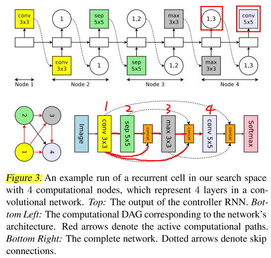
In this example, at layer k = 4, the controller samples previous indices {1, 3}, so the outputs of layers 1 and 3 are concatenated along their depth dimension and sent to layer 4.
在k=4层,控制器RNN选择1,3作为输入,因此1,3层的输出contact后作为第4层的输入
Meanwhile, the decision of what computation operation to use sets a particular layer into convolution or average pooling or max pooing.
同时,控制器RNN预测要使用的操作(卷积/平均池化/最大池化)
The 6 operations available for the controller are:
convolutions with filter sizes 3 × 3 and 5 × 5,
depthwise-separable convolutionswith filter sizes 3×3 and 5×5 (Chollet, 2017), and
max pooling and average pooling of kernel size 3 × 3.
总共有6种可选操作:
3 × 3 and 5 × 5 卷积
3 × 3 and 5 × 5 深度可分离卷积
3 × 3 最大池化、平均池化
Making the described set of decisions for a total of L times, we can sample a network of L layers.
执行以上预测步骤L次,即可确定网络的L层
Since all decisions are independent, there are (6^L × 2^{L(L−1)/2}) networks in the search space.
(6^L) :每一层有6种操作可以选择,一共L层
(2^{L(L−1)/2}) :(sum_{k=1}^{L} 2^{k-1})
In our experiments, L = 12, resulting in (1.6 × 10^{29}) possible networks.
在我们的实验中,L=12,共有 (1.6 × 10^{29}) 种网络
Sec 2.4. Designing Convolutional Cells
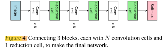
Rather than designing the entire convolutional network, one can design smaller modules and then connect them together to form a network.
不是直接搜索整个网络,而是先搜索cell,再堆叠cell
Figure 4 illustrates this design, where the convolutional cell and reduction cell architectures are to be designed.
以图4为例,说明conv cell 和 reduction cell是如何设计的
We utilize the ENAS computational DAG with B nodes to represent the computations that happen locally in a cell.
DAG是一个带有B个node的cell
In this DAG, node 1 and node 2 are treated as the cell’s inputs, which are the outputs of the two previous cells in the final network
在DAG中,当前cell 的 node 1 和 node 2表示cell的输入,来自之前2个cell的输出
For each of the remaining B − 2 nodes, we ask the controller RNN to make two sets of decisions:
two previous nodes to be used as inputs to the current node
two operations to apply to the two sampled nodes.
对于剩余的B-2个node(每个node有2个input,1个output),我们让控制器RNN做2个预测:
1)当前node的input取自哪两个之前的node
2)在2个input上施加什么操作
The 5 available operations are:
identity,
separable convolution with kernel size 3×3 and 5×5, and
average pooling and max pooling with kernel size 3×3.
5个可选操作:
identity
sep conv 3×3 and 5×5
avg pool 3×3、max pool 5×5
At each node, after the previous nodes and their corresponding operations are sampled, the operations are applied on the previous nodes, and their results are added.
每个node的2个input进行操作后,结果相加(add)
As before, we illustrate the mechanism of our search space with an example, here with B = 4 nodes (refer to Figure 5).
以图5为例说明cell搜索的过程,这里B=4,即每个cell有4个node
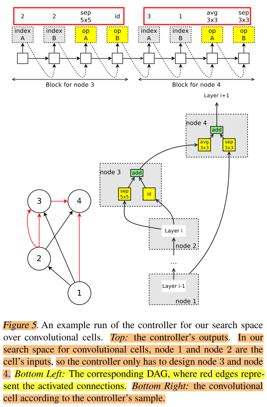
Details are as follows.
- Nodes 1, 2 are input nodes, so no decisions are needed for them. Let h1, h2 be the outputs of these nodes.
- At node 3: the controller samples two previous nodes and two operations. In Figure 5 Top Left, it samples node 2, node 2, separable conv 5x5, and identity. This means that h3 = sep conv 5x5(h2) + id(h2).
- At node 4: the controller samples node 3, node 1, avg pool 3x3, and sep conv 3x3. This means that h4 = avg pool 3x3(h3) + sep conv 3x3(h1).
- Since all nodes but h4 were used as inputs to at least another node, the only loose end, h4, is treated as the cell’s output. If there are multiple loose ends, they will be concatenated along the depth dimension to form the cell’s output.
- node 1 和 node 2 是输入节点,用h1,h2表示这两个节点的输出
- node 3:控制器RNN从当前node之前的node 选取2个作为输入,选中了2,2;选取2个操作,分别是sep 5x5 和 id,因此h3 = sep conv 5x5(h2) + id(h2)
- node4:控制器RNN从当前node之前的node 选取2个作为输入,选中了1,3;选取2个操作,分别是avg 3×3 和 sep 3×3,因此h4 = avg pool 3x3(h3) + sep conv 3x3(h1)
- cell中除了h4都被用作其他node的input,仅剩下h4未使用,因此将其作为cell的输出,如果有多个未使用的node的output,将这些output concat,一起作为cell的输出
A reduction cell can also be realized from the search space we discussed,
sampling a computational graph from the search space, and
applying all operations with a stride of 2.
reduction cell也可以使用同样的方法实现
1)从search space采样计算图
2)将stride设置为2
A reduction cell thus reduces the spatial dimensions of its input by a factor of 2.
因此reduction cell可以将feature map长宽降低为1/2
Following Zoph et al. (2018), we sample the reduction cell conditioned on the convolutional cell, hence making the controller RNN run for a total of 2(B − 2) blocks.
因此控制器RNN一共有2(B-2)个block
2(B-2):2种cell,每种cell 有 B 个node,但只有(B-2)个node需要决定,每个node有4个预测值(2个input,2个op)
Finally, we estimate the complexity of this search space.
最后估计search space 的复杂度
At node i (3 ≤ i ≤ B), the controller can select any two nodes from the i − 1 previous nodes, and any two operations from 5 operations.
第i(3 ≤ i ≤ B)个node,控制器RNN可以在之前i-1个node的outputs中抽样2次作为输入,从5中操作中抽样2次对应2个input的operation
As all decisions are independent, there are ((5 × (B − 2)!)^2) possible cells.
一共有 ((5 × (B − 2)!)^2) 种可能的cell
Since we independently sample for a convolutional cell and a reduction cell, the final size of the search space is ((5 × (B − 2)!)^4) .
如果独立预测conv cell 和 reduction cell,则共有 ((5 × (B − 2)!)^4) 种cell
With B = 7 as in our experiments, the search space can realize $ 1.3 × 10^{11}$ final networks, making it significantly smaller than the search space for entire convolutional networks (Section 2.3).
当B=7,即cell内有7个node时,共有 $ 1.3 × 10^{11}$ 中可能的网络,比2.3中的少很多
Experiments
Sec 3.2. Image Classification on CIFAR-10
We apply ENAS to two search spaces:
the macro search space over entire convolutional models (Section 2.3); and
the micro search space over convolutional cells (Section 2.4).
我们使用ENAS搜索2个搜索空间
1)整个网络
2)cell
Table 2 summarizes the test errors of ENAS and other approaches.
表2对比了ENAS与其他方法:
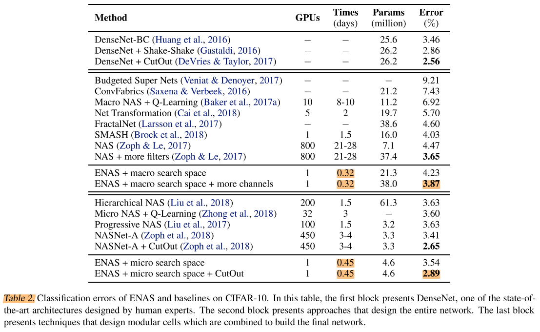
the first block presents the results of DenseNet (Huang et al., 2016), one of the highest-performing architectures that are designed by human experts.
表2的第一部分为DensNet,手工设计的最好的网络
The second block of Table 2 presents the performances of approaches that attempt to design an entire convolutional network, along with the the number of GPUs and the time these methods take to discover their final models.
表2的第二部分为ENAS与其他搜索整个网络的NAS方法对比
As shown, ENAS finds a network architecture, which we visualize in Figure 7, and which achieves 4.23% test error.
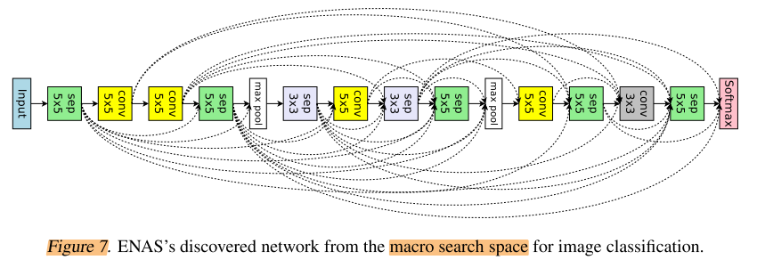
ENAS搜索到的整个网络结果如图7,达到4.23% err
If we keep the architecture, but increase the number of filters in the network’s highest layer to 512, then the test error decreases to 3.87%, which is not far away from NAS’s best model, whose test error is 3.65%.
如果使用同样的网络结构,将最后一层的filter数量增加到512,得到 3.87% err,比NAS的3.65%差距不大
Impressively, ENAS takes about 7 hours to find this architecture, reducing the number of GPU-hours by more than 50,000x compared to NAS.
重要的是,ENAS仅使用了7个gpu hours,比NAS方法快了50 000x
The third block of Table 2 presents the performances of approaches that attempt to design one more more modules and then connect them together to form the final networks.
表2的第3部分表示搜索cell再堆叠的方法的结果
ENAS takes 11.5 hours to discover the convolution cell and the reduction cell, which are visualized in Figure 8.
ENAS花费11.5hours 搜索到的 conv cell 和 reduction cell 如图8
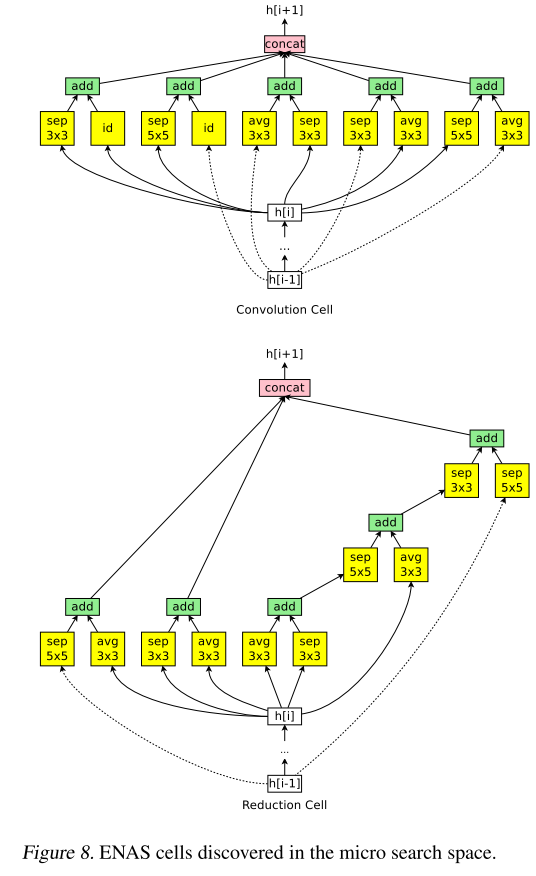
With the convolutional cell replicated for N = 6 times (c.f. Figure 4), ENAS achieves 3.54% test error, on par with the 3.41% error of NASNet-A (Zoph et al., 2018). With CutOut (DeVries & Taylor, 2017), ENAS’s error decreases to 2.89%, compared to 2.65% by NASNet-A.
conv cell的重复次数N=6,如图4,ENAS达到了 3.54% err,对应NASNet-A 的 3.41% err;使用cutout后,达到 2.89% err,对应NASNet-A 2.65% err
In addition to ENAS’s strong performance, we also find that the models found by ENAS are, in a sense, the local minimums in their search spaces.
ENAS搜索到的结构是搜索空间里的局部最小值
In particular, in the model that ENAS finds from the marco search space, if we replace all separable convolutions with normal convolutions, and then adjust the model size so that the number of parameters stay the same, then the test error increases by 1.7%.
在搜索整个网络的的结果中,将所有sep conv 替换为 conv,err增加了1.7%
Similarly, if we randomly change several connections in the cells that ENAS finds in the micro search space, the test error increases by 2.1%.
在搜索整个网络的的结果中,在搜索随机改变一些连接,err增加了2.1%
We thus believe that the controller RNN learned by ENAS is as good as the controller RNN learned by NAS, and that the performance gap between NAS and ENAS is due to the fact that we do not sample multiple architectures from our trained controller, train them, and then select the best architecture on the validation data. This extra step benefits NAS’s performance.
Sec 3.3. The Importance of ENAS
A question regarding ENAS’s importance is whether ENAS is actually capable of finding good architectures, or if it is the design of the search spaces that leads to ENAS’s strong empirical performance.
一个问题是,好的结果是搜索空间设计的原因,还是ENAS算法的原因?
Comparing to Guided Random Search
Our random convolutional network reaches 5.86% test error, and our two random cells reache 6.77% on CIFAR-10, while ENAS achieves 4.23% and 3.54%, respectively.
随机搜索整个网络和cell网络,err分别为5.86% 和 6.77%,使用ENAS后,分别是 4.23% 和 3.51%
Conclusion
However, NAS’s computational expense prevents it from being widely adopted.
NAS的计算开销使得它无法广泛应用
In this paper, we presented ENAS, a novel method that speeds up NAS by more than 1000x, in terms of GPU hours.
在本文中,我们提出ENAS,一种新的NAS算法,将gpu时间减少了1000x
ENAS’s key contribution is the sharing of parameters across child models during the search for architectures.
ENAS的主要贡献是在子网络之间权值共享
This insight is implemented by searching for a subgraph within a larger graph that incorporates architectures in a search space.
这是通过在大图中搜索子图来实现的,而大图就我们的搜索空间
We showed that ENAS works well on both CIFAR-10 and Penn Treebank datasets.