How to generate a sample from $p(x)$?
Let's first see how Matlab samples from a $p(x)$. In Matlab, there are several common probability distributions.

Try univariate Gaussian distribution
p= normpdf(linspace(xmin , xmax , num_of_points) , mean, standard_deviation);%PDF
c= normcdf(linspace(xmin , xmax , num_of_points) , mean, standard_deviation);%CDF
y=normrnd(mean, standard_deviation,number_of_samples, 1);%Random Number Generating Method
Try PDF:
x=linespace(-1,1,1000);
p=normpdf(x ,0, 1);
plot(x,p);
Note: linespace returns a vector which is usually accessed like this
x(1)%the first elem, not x(0)
x(:)
x(1,:)
Try RSM:
y=normrnd(0, 1,100, 1);%试试采10000个样本
hist( y , 20 );%20 bars
Try univariate uniform distribution
p= unifpdf(linspace(xmin , xmax , num_of_points) , a,b);%PDF
c= unifcdf(linspace(xmin , xmax , num_of_points) , a,b);%CDF
y=unifrnd(a,b,number_of_samples, 1);%RNG
Try PDF:
x=linespace(-10,10,1000);
p= unifpdf(x ,-5,5);
plot(x,p);
Try RSM:
y=unifrnd(-5, 5,100, 1);%试试采10000个样本
hist( y , 20 );%20 bars
Matlab provides random number generating functions for some standard $p(x)$, it doesn't provide us sampling functions for a general $p(x)$. Here I show some common sampling methods.
Inverse Transform Sampling(ITS)
with descret variables
This method generates random numbers from any probability distribution given the inverse of its cumulative distribution function. The idea is to sample uniformly distributed random numbers (between 0 and 1) and then transform these values using the inverse cumulative distribution function(InvCDF)(which can be descret or continous). If the InvCDF is descrete, then the ITS method just requires a table lookup, like shown in Table 1.
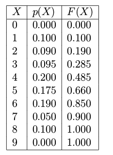
Table 1. Probability of digits observed in human random digit generation experiment
There is a method called randsample in Matlab that can implement the sampling process using the Table 1. See the code below.
%Note: The randsample doesn't defaultly exist in Octave-core package, install statistic package from http://octave.sourceforge.net/statistics/ before using randsample.

% probabilities for each digit
theta=[0.000; ... % digit 0
0.100; ... % digit 1
0.090; ... % digit 2
0.095; ... % digit 3
0.200; ... % digit 4
0.175; ... % digit 5
0.190; ... % digit 6
0.050; ... % digit 7
0.100; ... % digit 8
0.000];

seed = 1; rand( 'state' , seed );% fix the random number generator
K = 10000;% let's say we draw K random values
digitset = 0:9;
Y = randsample(digitset,K,true,theta);
figure( 1 ); clf;
counts = hist( Y , digitset );
bar( digitset , counts , 'k' );
xlim([-0.5 9.5]);
xlabel( 'Digit' );
ylabel( 'Frequency' );
title( 'Distribution of simulated draws of human digit generator' );
pause;
Instead of using the built-in functions such as randsample or mnrnd, it is helpful to consider how to implement the underlying sampling algorithm using the inverse transform method which is:
(1) Calculate $F(X)$.
(2) Sample u from Uniform(0,1).
(3) Get a sample $x^{i}$ of $P(X)$, which is $F(u)^{-1}$.
(4) Repeat (2) and (3) until we get enough samples.
Note: For discrete distributions, $F(X)^{-1}$ is discrete, the way to get a sample $x^{i}$ is illustrated below where $u=0.8,~x^{i}=6$ .

with continuous variables
This can be done with the following procedure:
(1) Draw U ∼ Uniform(0, 1).
(2) Set $X=F(U)^{-1}$
(3) Repeat
For example, we want to sample random numbers from the exponential distribution where its CDF is F (x|λ) = 1 − exp(−x/λ) . Then $F(u|gamma)^{-1}=-log(1-u)gamma$. Therefore replace $F(U)^{-1}$ with $F(u|gamma)^{-1}$.
p=-log(1-unifrnd(0,1,10000,1))*2;
hist(p,30);
Reject Sampling
Applied situation: impossible/difficult to compute CDF of $P(X)$.
Advantage: unlike MCMC, it doesn't require of any “burn-in” period, i.e., all samples obtained during sampling can immediately be used as samples from the target distribution $p( heta)$.

Based on the Figure above, the method is:
(1) Choose a proposal distribution q(θ) that is easy to sample from.
(2) Find a constant c such that cq(θ) ≥ p(θ) for all θ.
(3) Draw a proposal θ from q(θ).
(4) Draw a u from Uniform[0, cq(θ)].
(5) Reject the proposal if u > p(θ), accept otherwise. Actually, since u is sampled from Uniform[0, cq(θ)], it is equal to state like this " Reject if $uin[p( heta),cq( heta)]$, accept otherwise".
(6) Repeat steps 3, 4, and 5 until desired number of samples is reached; each accepted sample $ heta$ is a draw from p(θ).
For example

then the code is
k=100000;%draw k samples
c=2;
theta_vec=unifrnd(0,1,k,1)%gen a proposal vector from q($	heta$)
cq_vec=c*unifpdf(theta_vec);%cq(theta) vector
p_vec=2*theta_vec;%p(theta) vector
u_vec=[];
for cq=cq_vec
u_vec=[u_vec;unifrnd(0,cq)];
end
r=theta_vec.*(u_vec<p_vec);
r(r==0)=[];%remove the “0” elements
hist(r,20);

MCMC Sampling
Before getting to know MCMC sampling, we first get to know Monte Carlo Integration and Markov Chain.


For example:
%Implement the Markov Chain involving x under Beta(200(0.9x^((t-1))+0.05),200(1-0.9x^((t-1)-0.05))

fa=inline('','x')%parameter a for beta
fb=inline('200*(1-0.9*x-0.05)','x');%parameter b for beta
no4mc=4;%4 markove chains
states=unifrnd(0,1,1,no4mc);%initial states
N=1000;%200 samples drawn from 4 chains
X=states;
for i=1:N
states=betarnd(fa(states),fb(states));
X=[X;states];
end;
plot(X);
pause;
