1.2.1 Inverse transform sampling(ITS) with discrete variables
This method generates random numbers from any probability distribution given the inverse of its cumulative distribution function. The idea is to sample uniformly distributed random numbers (between 0 and 1) and then transform these values using the inverse cumulative distribution function(InvCDF)(which can be descret or continous). If the InvCDF is descrete, then the ITS method just requires a table lookup, like shown in Table 1.
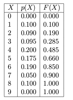
Table 1. Probability of digits observed in human random digit generation experiment
There is a method called randsample in Matlab that can implement the sampling process using the Table 1. See the code below.
%Note: The randsample doesn't defaultly exist in Octave-core package, install statistic package from http://octave.sourceforge.net/statistics/ before using randsample.

% probabilities for each digit
theta=[0.000; ... % digit 0
0.100; ... % digit 1
0.090; ... % digit 2
0.095; ... % digit 3
0.200; ... % digit 4
0.175; ... % digit 5
0.190; ... % digit 6
0.050; ... % digit 7
0.100; ... % digit 8
0.000];

seed = 1; rand( 'state' , seed );% fix the random number generator
K = 10000;% let's say we draw K random values
digitset = 0:9;
Y = randsample(digitset,K,true,theta);
figure( 1 ); clf;
counts = hist( Y , digitset );
bar( digitset , counts , 'k' );
xlim([-0.5 9.5]);
xlabel( 'Digit' );
ylabel( 'Frequency' );
title( 'Distribution of simulated draws of human digit generator' );
pause;
Instead of using the built-in functions such as randsample or mnrnd, it is helpful to consider how to implement the underlying sampling algorithm using the inverse transform method which is:
(1) Calculate $F(X)$.
(2) Sample u from Uniform(0,1).
(3) Get a sample $x^{i}$ of $P(X)$, which is $F(u)^{-1}$.
(4) Repeat (2) and (3) until we get enough samples.
Note: For discrete distributions, $F(X)^{-1}$ is discrete, the way to get a sample $x^{i}$ is illustrated below where $u=0.8,~x^{i}=6$ .

1.2.2 Inverse transform sampling with continuous variables
This can be done with the following procedure:
(1) Draw U ∼ Uniform(0, 1).
(2) Set $X=F(U)^{-1}$
(3) Repeat
For example, we want to sample random numbers from the exponential distribution where its CDF is F (x|λ) = 1 − exp(−x/λ) . Then $F(u|gamma)^{-1}=-log(1-u)gamma$. Therefore replace $F(U)^{-1}$ with $F(u|gamma)^{-1}$.
1.2.3 Rejection sampling
Applied situation: impossible/difficult to compute CDF of $P(X)$.
Advantage: unlike MCMC, it doesn't require of any “burn-in” period, i.e., all samples obtained during sampling can immediately be used as samples from the target distribution $p( heta)$.

Based on the Figure above, the method is:
(1) Choose a density q(θ) that is easy to sample from.
(2) Find a constant c such that cq(θ) ≥ p(θ) for all θ.
(3) Sample a proposal θ from proposal distribution q(θ).
(4) Sample a u from Uniform[0, cq(θ)].
(5) Reject the proposal if u > p(θ), accept otherwise. Actually, since u is sampled from Uniform[0, cq(θ)], it is equal to state like this " Reject if $uin[p( heta),cq( heta)]$, accept otherwise".
(6) Repeat steps 3, 4, and 5 until desired number of samples is reached; each accepted sample $ heta$ is a draw from p(θ).