时间序列预测案例一: 正弦波
PyTorch 官方给出了时间序列的预测案例:
https://github.com/pytorch/examples/tree/master/time_sequence_prediction
这是一个初学者上手的例子。它有助于学习pytorch和时间序列预测。本例中使用两个LSTMCell单元来学习从不同相位开始的一些正弦波信号。在学习了正弦波之后,网络试图预测未来的信号值。结果如下图所示。
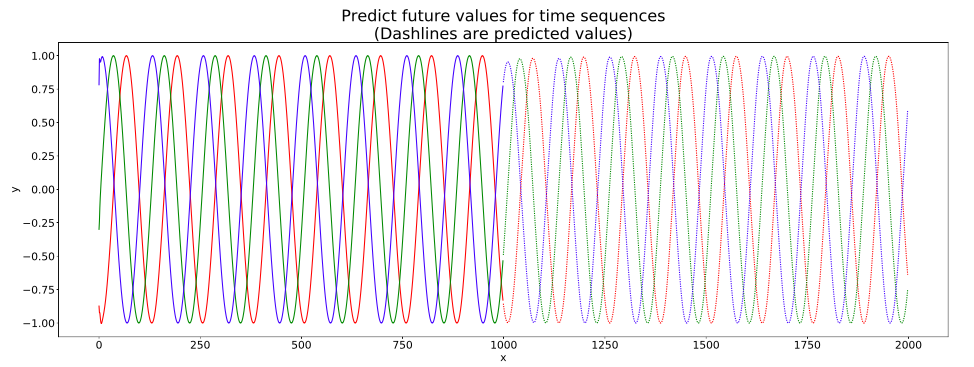
初始信号和预测结果如图所示。我们首先给出一些初始信号(实线)。网络随后将给出一些预测结果(虚线)。可以得出结论,该网络可以进行时间序列的预测。
import torch
import torch.nn as nn
import torch.optim as optim
import numpy as np
import matplotlib
# Non-interactive backend, you can't call plt.show() to see the figure interactively
# matplotlib.use('Agg') must be placed before import matplotlib.pyplot
matplotlib.use('Agg')
import matplotlib.pyplot as plt

device = torch.device("cuda:0" if torch.cuda.is_available() else "cpu")

def generateSineWave():
    np.random.seed(2)
    T = 20
    L = 1000
    N = 100
    x = np.empty((N, L), 'int64') #the dataset has 100 items and each item's length is 1000
    x[:] = np.array(range(L)) + np.random.randint(-4 * T, 4 * T, N).reshape(N, 1)
    data = np.sin(x / 1.0 / T).astype('float64')
    torch.save(data, open('traindata.pt', 'wb'))

class Sequence(nn.Module):
    def __init__(self):
        super(Sequence, self).__init__()
        self.lstm1 = nn.LSTMCell(1, 51)
        self.lstm2 = nn.LSTMCell(51, 51)
        self.linear = nn.Linear(51, 1)

    def forward(self, input, future = 0):
        outputs = []
        h_t = torch.zeros(input.size(0), 51, dtype=torch.double)
        c_t = torch.zeros(input.size(0), 51, dtype=torch.double)
        h_t2 = torch.zeros(input.size(0), 51, dtype=torch.double)
        c_t2 = torch.zeros(input.size(0), 51, dtype=torch.double)

        h_t = h_t.to(device)
        c_t = c_t.to(device)
        h_t2 = h_t2.to(device)
        c_t2 = c_t2.to(device)

        for i, input_t in enumerate(input.chunk(input.size(1), dim=1)):
            h_t, c_t = self.lstm1(input_t, (h_t, c_t))
            h_t2, c_t2 = self.lstm2(h_t, (h_t2, c_t2))
            output = self.linear(h_t2)  # output.shape:[batch,1]
            outputs += [output] # outputs.shape:[[batch,1],...[batch,1]], list composed of n [batch,1],
        for i in range(future):# if we should predict the future
            h_t, c_t = self.lstm1(output, (h_t, c_t))
            h_t2, c_t2 = self.lstm2(h_t, (h_t2, c_t2))
            output = self.linear(h_t2) # output.shape:[batch,1]
            outputs += [output]  # outputs.shape:[[batch,1],...[batch,1]], list composed of n [batch,1],
        outputs = torch.stack(outputs, 1).squeeze(2) # shape after stack:[batch, n, 1], shape after squeeze: [batch,n]
        return outputs


if __name__ == '__main__':
    # 1. generate sine wave data
    generateSineWave()
    # set random seed to 0
    np.random.seed(0)
    torch.manual_seed(0)
    # load data and make training set
    data = torch.load('traindata.pt')
    input = torch.from_numpy(data[3:, :-1])
    target = torch.from_numpy(data[3:, 1:])
    test_input = torch.from_numpy(data[:3, :-1])
    test_target = torch.from_numpy(data[:3, 1:])
    input = input.to(device)
    target = target.to(device)
    test_input = test_input.to(device)
    test_target = test_target.to(device)
    # 2. build the model
    seq = Sequence()
    seq.double()
    print(seq)
    # move to cuda
    # if torch.cuda.device_count()>1:
    #     seq = nn.DataParallel(seq)
    seq = seq.to(device)

    # 3 loss function
    criterion = nn.MSELoss()
    # 4 use LBFGS as optimizer since we can load the whole data to train
    optimizer = optim.LBFGS(seq.parameters(), lr=0.8)
    # 5 begin to train
    for i in range(1):
        print('STEP: ', i)
        def closure():
            # forward
            out = seq(input)
            loss = criterion(out, target)
            print('loss:', loss.item())
            # backward
            optimizer.zero_grad()
            loss.backward()
            return loss
        optimizer.step(closure)
        # begin to predict, no need to track gradient here
        with torch.no_grad():
            future = 1000
            pred = seq(test_input, future=future)
            loss = criterion(pred[:, :-future], test_target)
            print('test loss:', loss.item())

            y = pred.detach().cpu()
            y = y.numpy()
        # draw the result
        plt.figure(figsize=(30,10))
        plt.title('Predict future values for time sequences
(Dashlines are predicted values)', fontsize=30)
        plt.xlabel('x', fontsize=20)
        plt.ylabel('y', fontsize=20)
        plt.xticks(fontsize=20)
        plt.yticks(fontsize=20)
        def draw(yi, color):
            plt.plot(np.arange(input.size(1)), yi[:input.size(1)], color, linewidth = 2.0)
            plt.plot(np.arange(input.size(1), input.size(1) + future), yi[input.size(1):], color + ':', linewidth = 2.0)
        draw(y[0], 'r')
        draw(y[1], 'g')
        draw(y[2], 'b')
        plt.savefig('predict%d.pdf'%i)
        plt.close()
时间序列预测案例二: 股票预测
原文地址: https://www.7forz.com/3319/
学习使用 LSTM 来预测时间序列,本文中使用上证指数的收盘价。
首先用 tushare 下载上证指数的K线数据,然后作标准化处理。
import numpy as np
import tushare as ts
data_close = ts.get_k_data('000001', start='2018-01-01', index=True)['close'].values  # 获取上证指数从20180101开始的收盘价的np.ndarray
data_close = data_close.astype('float32')  # 转换数据类型
# 将价格标准化到0~1
max_value = np.max(data_close)
min_value = np.min(data_close)
data_close = (data_close - min_value) / (max_value - min_value)
原始数据:上证指数从2018-01-01到2019-05-24的收盘价(未标准化处理)
把K线数据进行分割,每 DAYS_FOR_TRAIN 个收盘价对应 1 个未来的收盘价。例如K线为 [1,2,3,4,5], DAYS_FOR_TRAIN=3,那么将会生成2组数据:
第1组的输入是 [1,2,3],对应输出 4;
第2组的输入是 [2,3,4],对应输出 5。
然后只使用前70%的数据用于训练,剩下的不用,用来与实际数据进行对比。
DAYS_FOR_TRAIN = 10

def create_dataset(data, days_for_train=5) -> (np.array, np.array):
    """
        根据给定的序列data,生成数据集

        数据集分为输入和输出,每一个输入的长度为days_for_train,每一个输出的长度为1。
        也就是说用days_for_train天的数据,对应下一天的数据。

        若给定序列的长度为d,将输出长度为(d-days_for_train+1)个输入/输出对
    """
    dataset_x, dataset_y= [], []
    for i in range(len(data)-days_for_train):
        _x = data[i:(i+days_for_train)]
        dataset_x.append(_x)
        dataset_y.append(data[i+days_for_train])
    return (np.array(dataset_x), np.array(dataset_y))

dataset_x, dataset_y = create_dataset(data_close, DAYS_FOR_TRAIN)

# 划分训练集和测试集,70%作为训练集
train_size = int(len(dataset_x) * 0.7)

train_x = dataset_x[:train_size]
train_y = dataset_y[:train_size]

# 将数据改变形状,RNN 读入的数据维度是 (seq_size, batch_size, feature_size)
train_x = train_x.reshape(-1, 1, DAYS_FOR_TRAIN)
train_y = train_y.reshape(-1, 1, 1)


# 转为pytorch的tensor对象
train_x = torch.from_numpy(train_x)
train_y = torch.from_numpy(train_y)
定义网络、优化器、loss函数
import torch
from torch import nn
class LSTM_Regression(nn.Module):
    """
        使用LSTM进行回归

        参数:
        - input_size: feature size
        - hidden_size: number of hidden units
        - output_size: number of output
        - num_layers: layers of LSTM to stack
    """
    def __init__(self, input_size, hidden_size, output_size=1, num_layers=2):
        super().__init__()
        self.lstm = nn.LSTM(input_size, hidden_size, num_layers)
        self.fc = nn.Linear(hidden_size, output_size)
    def forward(self, _x):
        x, _ = self.lstm(_x)  # _x is input, size (seq_len, batch, input_size)
        s, b, h = x.shape  # x is output, size (seq_len, batch, hidden_size)
        x = x.view(s*b, h)
        x = self.fc(x)
        x = x.view(s, b, -1)  # 把形状改回来
        return x
model = LSTM_Regression(DAYS_FOR_TRAIN, 8, output_size=1, num_layers=2)
loss_function = nn.MSELoss()
optimizer = torch.optim.Adam(model.parameters(), lr=1e-2)
训练
for i in range(1000):
    out = model(train_x)
    loss = loss_function(out, train_y)
    loss.backward()
    optimizer.step()
    optimizer.zero_grad()
    if (i+1) % 100 == 0:
        print('Epoch: {}, Loss:{:.5f}'.format(i+1, loss.item()))
测试
import matplotlib.pyplot as plt
model = model.eval() # 转换成测试模式
# 注意这里用的是全集 模型的输出长度会比原数据少DAYS_FOR_TRAIN 填充使长度相等再作图
dataset_x = dataset_x.reshape(-1, 1, DAYS_FOR_TRAIN)  # (seq_size, batch_size, feature_size)
dataset_x = torch.from_numpy(dataset_x)
pred_test = model(dataset_x) # 全量训练集的模型输出 (seq_size, batch_size, output_size)
pred_test = pred_test.view(-1).data.numpy()
pred_test = np.concatenate((np.zeros(DAYS_FOR_TRAIN), pred_test))  # 填充0 使长度相同
assert len(pred_test) == len(data_close)
plt.plot(pred_test, 'r', label='prediction')
plt.plot(data_close, 'b', label='real')
plt.plot((train_size, train_size), (0, 1), 'g--')
plt.legend(loc='best')
plt.show()