kaggle数据地址:https://www.kaggle.com/sakshigoyal7/credit-card-customers
导入数据
#导入模块
import pandas as pd
import numpy as np
import  matplotlib.pyplot as plt
import seaborn as sns

BankChurners = pd.read_csv('D:\python_home\预测客户流失\bankchurners\BankChurners.csv')
简单的数据查看
BankChurners.columns

'''
Index(['CLIENTNUM', 'Attrition_Flag', 'Customer_Age', 'Gender',
       'Dependent_count', 'Education_Level', 'Marital_Status',
       'Income_Category', 'Card_Category', 'Months_on_book',
       'Total_Relationship_Count', 'Months_Inactive_12_mon',
       'Contacts_Count_12_mon', 'Credit_Limit', 'Total_Revolving_Bal',
       'Avg_Open_To_Buy', 'Total_Amt_Chng_Q4_Q1', 'Total_Trans_Amt',
       'Total_Trans_Ct', 'Total_Ct_Chng_Q4_Q1', 'Avg_Utilization_Ratio',
       'Naive_Bayes_Classifier_Attrition_Flag_Card_Category_Contacts_Count_12_mon_Dependent_count_Education_Level_Months_Inactive_12_mon_1',
       'Naive_Bayes_Classifier_Attrition_Flag_Card_Category_Contacts_Count_12_mon_Dependent_count_Education_Level_Months_Inactive_12_mon_2'],
      dtype='object')
'''
拿到百度翻译了一下
'''
'CLIENTNUM','消耗标志','客户年龄','性别',

“受抚养人数量”、“受教育程度”、“婚姻状况”,

'收入类别','卡片类别','账面上的月份',

'总关系数','月数'u不活跃'u 12个月',

“联系人数量12个月”,“信用额度”,“总周转余额”,

'平均开盘价到买入价','总金额',

'总交易量','第4季度总交易量','平均利用率',

'天真的_Bayes_分类器_消耗_标志_卡片_类别_联系人_Count_12 _mon_依赖性_Count_u教育程度_u个月_不活跃_12 _mon_1',

'天真的_Bayes_分类器_消耗_标志_卡片_类别_联系人_Count_12 _mon_依赖性_Count_受教育程度_u月_不活跃_12_mon_2'],

dtype='object'
'''
简单看一下缺失情况
#木有空值,但是不代表没有其他表达类型的空值,比如说'-'
BankChurners.isnull().sum()
我们按照数据类型分一下字段
#数据特征
numeric_features = BankChurners.select_dtypes(include=[np.number])
print(numeric_features.columns)
#类别特征
categorical_features = BankChurners.select_dtypes(include=[np.object])
print(categorical_features.columns)
Index(['CLIENTNUM', 'Customer_Age', 'Dependent_count', 'Months_on_book',
       'Total_Relationship_Count', 'Months_Inactive_12_mon',
       'Contacts_Count_12_mon', 'Credit_Limit', 'Total_Revolving_Bal',
       'Avg_Open_To_Buy', 'Total_Amt_Chng_Q4_Q1', 'Total_Trans_Amt',
       'Total_Trans_Ct', 'Total_Ct_Chng_Q4_Q1', 'Avg_Utilization_Ratio',
       'Naive_Bayes_Classifier_Attrition_Flag_Card_Category_Contacts_Count_12_mon_Dependent_count_Education_Level_Months_Inactive_12_mon_1',
       'Naive_Bayes_Classifier_Attrition_Flag_Card_Category_Contacts_Count_12_mon_Dependent_count_Education_Level_Months_Inactive_12_mon_2'],
      dtype='object')
Index(['Attrition_Flag', 'Gender', 'Education_Level', 'Marital_Status',
       'Income_Category', 'Card_Category'],
      dtype='object')
看看类别型变量的唯一值
for i in list(categorical_features.columns):
    print('*************************')
    print('{0}+的唯一值如下:{1}'.format(i,BankChurners[i].nunique()))
    print(BankChurners[i].unique())
*************************
Attrition_Flag+的唯一值如下:2
['Existing Customer' 'Attrited Customer']
*************************
Gender+的唯一值如下:2
['M' 'F']
*************************
Education_Level+的唯一值如下:7
['High School' 'Graduate' 'Uneducated' 'Unknown' 'College' 'Post-Graduate'
 'Doctorate']
*************************
Marital_Status+的唯一值如下:4
['Married' 'Single' 'Unknown' 'Divorced']
*************************
Income_Category+的唯一值如下:6
['$60K - $80K' 'Less than $40K' '$80K - $120K' '$40K - $60K' '$120K +'
 'Unknown']
*************************
Card_Category+的唯一值如下:4
['Blue' 'Gold' 'Silver' 'Platinum']
看来没有乱七八糟的空值
我们在看一下数值型变量的分布
plt.figure(figsize=(20,50))
col = list(numeric_features.columns)
for i in range(1,len(numeric_features.columns)+1):
    ax=plt.subplot(9,2,i)
    sns.kdeplot(BankChurners[col[i-1]],bw=1.5)
    plt.xlabel(col[i-1])
plt.show()
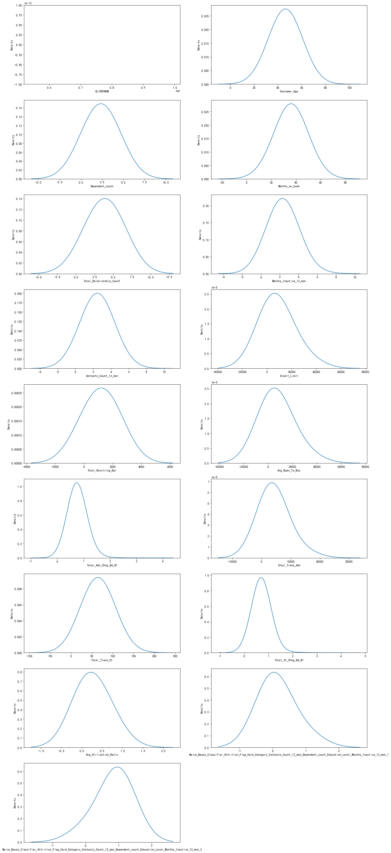
我们看上面变量,第一个变量CLIENTNUM 其实就是客户ID,我们可以不用理会
仔细看上面的图片,我们就会发现,其实有些字段其实是类别比较少的数值型变量,但是还是写代码看好,眼睛有时也会出卖自己
for i in list(numeric_features.columns):
    print('{0}+的唯一值如下:{1}'.format(i,BankChurners[i].nunique()))
CLIENTNUM+的唯一值如下:10127
Customer_Age+的唯一值如下:45
Dependent_count+的唯一值如下:6
Months_on_book+的唯一值如下:44
Total_Relationship_Count+的唯一值如下:6
Months_Inactive_12_mon+的唯一值如下:7
Contacts_Count_12_mon+的唯一值如下:7
Credit_Limit+的唯一值如下:6205
Total_Revolving_Bal+的唯一值如下:1974
Avg_Open_To_Buy+的唯一值如下:6813
Total_Amt_Chng_Q4_Q1+的唯一值如下:1158
Total_Trans_Amt+的唯一值如下:5033
Total_Trans_Ct+的唯一值如下:126
Total_Ct_Chng_Q4_Q1+的唯一值如下:830
Avg_Utilization_Ratio+的唯一值如下:964
Naive_Bayes_Classifier_Attrition_Flag_Card_Category_Contacts_Count_12_mon_Dependent_count_Education_Level_Months_Inactive_12_mon_1+的唯一值如下:1704
Naive_Bayes_Classifier_Attrition_Flag_Card_Category_Contacts_Count_12_mon_Dependent_count_Education_Level_Months_Inactive_12_mon_2+的唯一值如下:640
我们把它归为一类
num_cate_col = [  'Dependent_count',
       'Total_Relationship_Count', 'Months_Inactive_12_mon',
       'Contacts_Count_12_mon',
       ]
剩下的归为一类
numeric_col = [ x for x in list(numeric_features.columns) if x not in num_cate_col]
numeric_col.remove('CLIENTNUM')
numeric_col
'''
['Customer_Age',
 'Months_on_book',
 'Credit_Limit',
 'Total_Revolving_Bal',
 'Avg_Open_To_Buy',
 'Total_Amt_Chng_Q4_Q1',
 'Total_Trans_Amt',
 'Total_Trans_Ct',
 'Total_Ct_Chng_Q4_Q1',
 'Avg_Utilization_Ratio',
 'Naive_Bayes_Classifier_Attrition_Flag_Card_Category_Contacts_Count_12_mon_Dependent_count_Education_Level_Months_Inactive_12_mon_1',
 'Naive_Bayes_Classifier_Attrition_Flag_Card_Category_Contacts_Count_12_mon_Dependent_count_Education_Level_Months_Inactive_12_mon_2']
'''
我们在看看类别比较少的数值型变量
for i in num_cate_col:
    print('*************************')
    print('{0}+的唯一值如下:{1}'.format(i,BankChurners[i].nunique()))
    print(BankChurners[i].unique())
*************************
Dependent_count+的唯一值如下:6
[3 5 4 2 0 1]
*************************
Total_Relationship_Count+的唯一值如下:6
[5 6 4 3 2 1]
*************************
Months_Inactive_12_mon+的唯一值如下:7
[1 4 2 3 6 0 5]
*************************
Contacts_Count_12_mon+的唯一值如下:7
[3 2 0 1 4 5 6]
看看y值Attrition_Flag
BankChurners['Attrition_Flag'].value_counts().plot.pie(explode=[0,0.1],autopct='%1.1f%%')
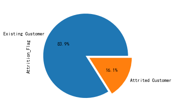
比例为16%,还好
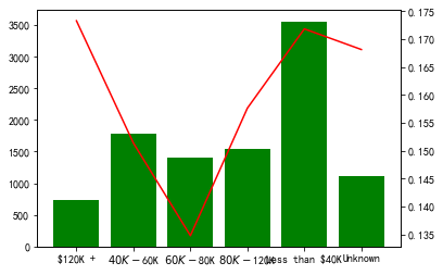
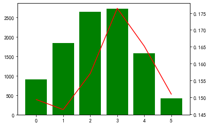
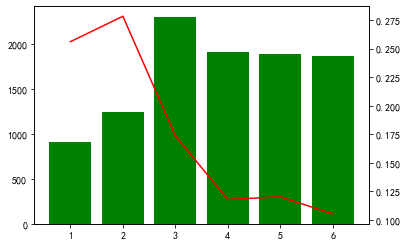
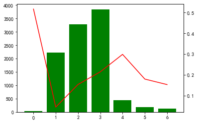
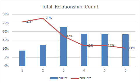
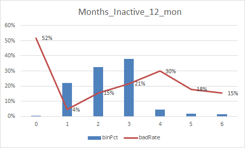
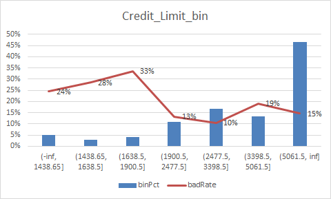
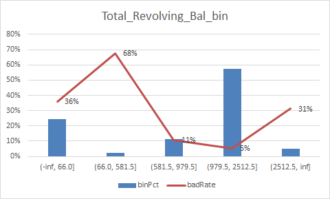
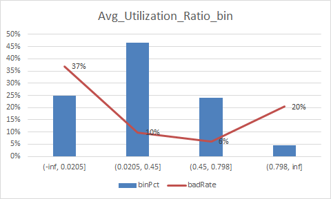
画类别变量的直方图以及逾期概率图
cate_cold = list(categorical_features.columns)+num_cate_col
for i in cate_cold:
    tmp = pd.crosstab(BankChurners[i], BankChurners['Attrition_Flag'])
    tmp['总人数'] = tmp.sum(axis=1)
    tmp['流失率'] = tmp['Attrited Customer']/tmp['总人数']
    fig, ax1 = plt.subplots()
    ax1.bar(tmp.index,tmp['总人数'],color='green')
    ax2 = ax1.twinx()
    ax2.plot(tmp.index,tmp['流失率'],color='red')
    plt.show()


构建特征
2021.1.15来补充一下建模的部分
具体过程就不写了,直接附上代码,以及结果
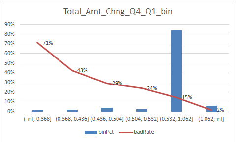
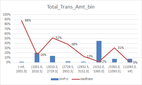
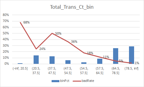
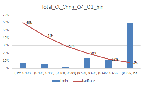
# -*- coding: utf-8 -*-
"""
Created on Fri Jan 15 09:18:46 2021

@author: Administrator
"""

import pandas as pd
import numpy as np
import  matplotlib.pyplot as plt
import seaborn as sns
import pycard as pc

#%%导入数据
BankChurners = pd.read_csv('D:\python_home\预测客户流失\bankchurners\BankChurners.csv')

BankChurners.isnull().sum()

#%%区分数值型变量和类别型变量
num_col = ['Customer_Age',
 'Months_on_book',
 'Credit_Limit',
 'Total_Revolving_Bal',
 'Avg_Open_To_Buy',
 'Total_Amt_Chng_Q4_Q1',
 'Total_Trans_Amt',
 'Total_Trans_Ct',
 'Total_Ct_Chng_Q4_Q1',
 'Avg_Utilization_Ratio',
 'Naive_Bayes_Classifier_Attrition_Flag_Card_Category_Contacts_Count_12_mon_Dependent_count_Education_Level_Months_Inactive_12_mon_1',
 'Naive_Bayes_Classifier_Attrition_Flag_Card_Category_Contacts_Count_12_mon_Dependent_count_Education_Level_Months_Inactive_12_mon_2']


cate_col = [ i for i in list(BankChurners.columns) if i not in num_col]
cate_col.remove('CLIENTNUM')
cate_col
'''
['Attrition_Flag',
 'Gender',
 'Dependent_count',
 'Education_Level',
 'Marital_Status',
 'Income_Category',
 'Card_Category',
 'Total_Relationship_Count',
 'Months_Inactive_12_mon',
 'Contacts_Count_12_mon']
'''

#%%cate_col.unqion()
for i in cate_col:
    print(i,BankChurners[i].unique())
'''
Attrition_Flag ['Existing Customer' 'Attrited Customer']
Gender ['M' 'F']
Dependent_count [3 5 4 2 0 1]
Education_Level ['High School' 'Graduate' 'Uneducated' 'Unknown' 'College' 'Post-Graduate'
 'Doctorate']
Marital_Status ['Married' 'Single' 'Unknown' 'Divorced']
Income_Category ['$60K - $80K' 'Less than $40K' '$80K - $120K' '$40K - $60K' '$120K +'
 'Unknown']
Card_Category ['Blue' 'Gold' 'Silver' 'Platinum']
Total_Relationship_Count [5 6 4 3 2 1]
Months_Inactive_12_mon [1 4 2 3 6 0 5]
Contacts_Count_12_mon [3 2 0 1 4 5 6]
'''

#%%处理目标变量,赋值0和1 流失就是1
BankChurners.Attrition_Flag = BankChurners.Attrition_Flag.map({'Existing Customer':0,'Attrited Customer':1})


#%%类别变量的iv计算
cate_iv_woedf = pc.WoeDf()
clf = pc.NumBin()
for i in cate_col[1:]:
    cate_iv_woedf.append(pc.cross_woe(BankChurners[i] ,BankChurners.Attrition_Flag))
cate_iv_woedf.to_excel('tmp11')


#尝试使用二者组合变量,发现并没有作用
BankChurners['Gender_Dependent_count'] = BankChurners.apply(lambda x :x.Gender+ str(x.Dependent_count),axis=1)
pc.cross_woe(BankChurners.Gender_Dependent_count,BankChurners.Attrition_Flag)
BankChurners['Education_Level_Income_Category'] = BankChurners.apply(lambda x :x.Education_Level+ str(x.Income_Category),axis=1)
pc.cross_woe(BankChurners.Education_Level_Income_Category,BankChurners.Attrition_Flag)
BankChurners.pop('Gender_Dependent_count')
BankChurners.pop('Education_Level_Income_Category')

#%%数值变量的iv值计算
num_iv_woedf = pc.WoeDf()
clf = pc.NumBin()
for i in num_col:
    clf.fit(BankChurners[i] ,BankChurners.Attrition_Flag)
    clf.generate_transform_fun()
    num_iv_woedf.append(clf.woe_df_)
num_iv_woedf.to_excel('tmp12')

#%%简单处理一下变量
#Total_Relationship_Count,Months_Inactive_12_mon,Contacts_Count_12_mon,类别型变量就不需要管了,保留原来的分区即可


#Credit_Limit
from numpy import *
BankChurners['Credit_Limit_bin'] = pd.cut(BankChurners.Credit_Limit,bins=[-inf, 1438.65, 1638.5, 1900.5, 2477.5, 3398.5, 5061.5, inf])
BankChurners['Total_Revolving_Bal_bin'] = pd.cut(BankChurners.Total_Revolving_Bal,bins=[-inf, 66.0, 581.5, 979.5, 2512.5, inf])
BankChurners['Avg_Open_To_Buy_bin'] = pd.cut(BankChurners.Avg_Open_To_Buy,bins=[-inf, 447.5, 1038.5, 1437.0, 1944.5, 2229.5,  inf])
BankChurners['Total_Amt_Chng_Q4_Q1_bin'] = pd.cut(BankChurners.Total_Amt_Chng_Q4_Q1,bins=[-inf,  0.3685, 0.4355, 0.5045, 0.5325, 1.0625, inf])
BankChurners['Total_Trans_Amt_bin'] = pd.cut(BankChurners.Total_Trans_Amt,bins=[-inf, 1001.0, 2010.5, 2729.5, 2932.5, 3152.0, 5365.0, 11093.0, inf])
BankChurners['Total_Trans_Ct_bin'] = pd.cut(BankChurners.Total_Trans_Ct,bins=[-inf, 20.5, 37.5, 47.5, 54.5, 57.5, 64.5, 78.5, inf])
BankChurners['Total_Ct_Chng_Q4_Q1_bin'] = pd.cut(BankChurners.Total_Ct_Chng_Q4_Q1,bins=[-inf, 0.4075,  0.4875, 0.504, 0.6015, 0.6565, inf])
BankChurners['Avg_Utilization_Ratio_bin'] = pd.cut(BankChurners.Avg_Utilization_Ratio,bins=[-inf,  0.0205, 0.4505, 0.7985,  inf])
BankChurners['Naive_Bayes1_bin'] = pd.cut(BankChurners.Naive_Bayes_Classifier_Attrition_Flag_Card_Category_Contacts_Count_12_mon_Dependent_count_Education_Level_Months_Inactive_12_mon_1,
                                         bins=[-inf, 0.4736, inf])
BankChurners['Naive_Bayes2_bin'] = pd.cut(BankChurners.Naive_Bayes_Classifier_Attrition_Flag_Card_Category_Contacts_Count_12_mon_Dependent_count_Education_Level_Months_Inactive_12_mon_2,
                                         bins=[-inf, 0.5264, inf])


iv_col = [i for i in ['Total_Relationship_Count','Months_Inactive_12_mon','Contacts_Count_12_mon',
          ] + list(BankChurners.columns)[-10:]]

cate_iv_woedf = pc.WoeDf()
clf = pc.NumBin()
for i in iv_col:
    cate_iv_woedf.append(pc.cross_woe(BankChurners[i] ,BankChurners.Attrition_Flag))
cate_iv_woedf.to_excel('tmp11')

BankChurners.Contacts_Count_12_mon[BankChurners.Contacts_Count_12_mon ==6] =5

#%%解决方案如下:
#解决方案:后面这两个就不入模型了,作为规则即可,不然会导致过拟合,上面的出现了无穷的变量要合并区间
iv_col = [i for i in ['Total_Relationship_Count','Months_Inactive_12_mon','Contacts_Count_12_mon',
          ] + list(BankChurners.columns)[-10:-2]]

cate_iv_woedf = pc.WoeDf()
clf = pc.NumBin()
for i in iv_col:
    cate_iv_woedf.append(pc.cross_woe(BankChurners[i] ,BankChurners.Attrition_Flag))
cate_iv_woedf.to_excel('tmp11')

#%%woe转换
pc.obj_info(cate_iv_woedf)

cate_iv_woedf.bin2woe(BankChurners,iv_col)

model_col = [i for i in ['CLIENTNUM', 'Attrition_Flag']+list(BankChurners.columns)[-11:]]

#%%建模
import pandas as pd
import matplotlib.pyplot as plt #导入图像库
import matplotlib
import seaborn as sns
import statsmodels.api as sm
from sklearn.metrics import roc_curve, auc
from sklearn.model_selection import train_test_split

X = BankChurners[list(BankChurners.columns)[-11:]]
Y = BankChurners['Attrition_Flag']


x_train,x_test,y_train,y_test=train_test_split(X,Y,test_size=0.3,random_state=0)

#(10127, 44)

X1=sm.add_constant(x_train)   #在X前加上一列常数1,方便做带截距项的回归
logit=sm.Logit(y_train.astype(float),X1.astype(float))
result=logit.fit()
result.summary()
result.params


X3 = sm.add_constant(x_test)
resu = result.predict(X3.astype(float))
fpr, tpr, threshold = roc_curve(y_test, resu)
rocauc = auc(fpr, tpr)
plt.plot(fpr, tpr, 'b', label='AUC = %0.2f' % rocauc)
plt.legend(loc='lower right')
plt.plot([0, 1], [0, 1], 'r--')
plt.xlim([0, 1])
plt.ylim([0, 1])
plt.ylabel('真正率')
plt.xlabel('假正率')
plt.show()
模型的参数如下:
const -1.662204
Total_Relationship_C_woe -2.307529
Months_Inactive_12_woe -1.050666
Contacts_Count_12_woe -0.742126
Credit_Limit_woe -0.633916
Total_Revolving_Bal_woe -0.914706
Avg_Open_To_Buy_woe -0.120073
Total_Amt_Chng_Q4_Q1_woe -0.845637
Total_Trans_Amt_woe -0.924220
Total_Trans_Ct_woe -0.601850
Total_Ct_Chng_Q4_Q1_woe -0.493193
Avg_Utilization_Ratio_woe -0.265479
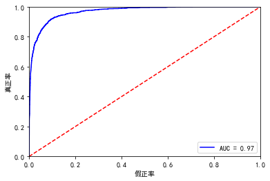
测试集的auc图片如下:
0.9651589169400466

看看训练集的auc
resu_1 = result.predict(X1.astype(float))
fpr, tpr, threshold = roc_curve(y_train, resu_1)
rocauc = auc(fpr, tpr)
plt.plot(fpr, tpr, 'b', label='AUC = %0.2f' % rocauc)
plt.legend(loc='lower right')
plt.plot([0, 1], [0, 1], 'r--')
plt.xlim([0, 1])
plt.ylim([0, 1])
plt.ylabel('真正率')
plt.xlabel('假正率')
plt.show()
0.9683602097734862
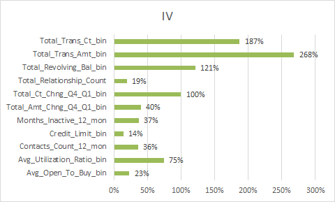
放一下入模变量的iv值


总结:
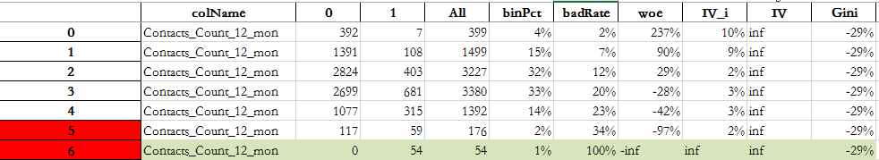
1.变量的逾期率不单调,没有关系,但是分箱时每个箱子不能太小,太小需要合并,最好挑选iv值比较好(2%以上)的入魔,使用woe去训练模型
2.关于iv值为无穷时候的做法:
IVi无论等于负无穷还是正无穷,都是没有意义的。
由上述问题我们可以看到,使用IV其实有一个缺点,就是不能自动处理变量的分组中出现响应比例为0或100%的情况。那么,遇到响应比例为0或者100%的情况,我们应该怎么做呢?建议如下:
(1)如果可能,直接把这个分组做成一个规则,作为模型的前置条件或补充条件;
(2)重新对变量进行离散化或分组,使每个分组的响应比例都不为0且不为100%,尤其是当一个分组个体数很小时(比如小于100个),强烈建议这样做,因为本身把一个分组个体数弄得很小就不是太合理。
(3)如果上面两种方法都无法使用,建议人工把该分组的响应数和非响应的数量进行一定的调整。如果响应数原本为0,可以人工调整响应数为1,如果非响应数原本为0,可以人工调整非响应数为1.
本次也出现了两种iv值为无穷的情况
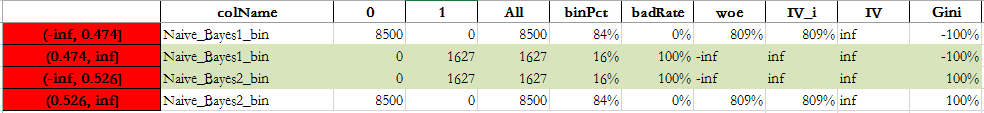
我的处理方法是:
解决方案:后面这两个就不入模型了,作为规则即可,不然可能导致过拟合,上面的出现了无穷的变量要合并区间
还有一些个人信息的特征,比如年龄,婚姻等等,由于iv值很低就没有放进去,但是还是值得探讨一下,不过本次的模型的效果很好,就不做太复杂的模型了
但是还有一个疑惑是:
Naive_Bayes_Classifier_Attrition_Flag_Card_Category_Contacts_Count_12_mon_Dependent_count_Education_Level_Months_Inactive_12_mon_1
Naive_Bayes_Classifier_Attrition_Flag_Card_Category_Contacts_Count_12_mon_Dependent_count_Education_Level_Months_Inactive_12_mon_2
最后两个变量实在是太厉害了,不知道是不是别人训练好的y?
需要查资料看看
最后在官网找到了答案