Part1 Demo实践
- Step1:库函数导入
- Step2:模型训练
- Step3:模型参数查看
- Step4:数据和模型可视化
- Step5:模型预测
Part2 基于鸢尾花(iris)数据集的逻辑回归分类实践
- Step1:库函数导入
- Step2:数据读取/载入
- Step3:数据信息简单查看
- Step4:可视化描述
- Step5:利用 逻辑回归模型 在二分类上 进行训练和预测
- Step6:利用 逻辑回归模型 在三分类(多分类)上 进行训练和预测
Demo实践
Step1:库函数导入
##  基础函数库
import numpy as np

## 导入画图库
import matplotlib.pyplot as plt
import seaborn as sns

## 导入逻辑回归模型函数
from sklearn.linear_model import LogisticRegression
Step2:训练模型
##Demo演示LogisticRegression分类

## 构造数据集
x_fearures = np.array([[-1, -2], [-2, -1], [-3, -2], [1, 3], [2, 1], [3, 2]])
y_label = np.array([0, 0, 0, 1, 1, 1])

## 调用逻辑回归模型
lr_clf = LogisticRegression()

## 用逻辑回归模型拟合构造的数据集
lr_clf = lr_clf.fit(x_fearures, y_label) #其拟合方程为 y=w0+w1*x1+w2*x2
Step3:模型参数查看
##查看其对应模型的w  参数
print('the weight of Logistic Regression:',lr_clf.coef_)
##查看其对应模型的w0  截距
print('the intercept(w0) of Logistic Regression:',lr_clf.intercept_)
##the weight of Logistic Regression:[[0.73462087 0.6947908]]
##the intercept(w0) of Logistic Regression:[-0.03643213]
Step4:数据和模型可视化
## 可视化构造的数据样本点
plt.figure()
plt.scatter(x_fearures[:,0],x_fearures[:,1], c=y_label, s=50, cmap='viridis')
plt.title('Dataset')
plt.show()

# 可视化决策边界
plt.figure()
plt.scatter(x_fearures[:,0],x_fearures[:,1], c=y_label, s=50, cmap='viridis')
plt.title('Dataset')

nx, ny = 200, 100
x_min, x_max = plt.xlim()  #返回x轴的范围
y_min, y_max = plt.ylim()  #返回y轴的范围
x_grid, y_grid = np.meshgrid(np.linspace(x_min, x_max, nx),np.linspace(y_min, y_max, ny))

z_proba = lr_clf.predict_proba(np.c_[x_grid.ravel(), y_grid.ravel()])
z_proba = z_proba[:, 1].reshape(x_grid.shape)
plt.contour(x_grid, y_grid, z_proba, [0.5], linewidths=2., colors='blue')

plt.show()

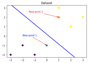
### 可视化预测新样本

plt.figure()
## new point 1
x_fearures_new1 = np.array([[0, -1]])
plt.scatter(x_fearures_new1[:,0],x_fearures_new1[:,1], s=50, cmap='viridis')
plt.annotate(s='New point 1',xy=(0,-1),xytext=(-2,0),color='blue',arrowprops=dict(arrowstyle='-|>',connectionstyle='arc3',color='red'))

## new point 2
x_fearures_new2 = np.array([[1, 2]])
plt.scatter(x_fearures_new2[:,0],x_fearures_new2[:,1], s=50, cmap='viridis')
plt.annotate(s='New point 2',xy=(1,2),xytext=(-1.5,2.5),color='red',arrowprops=dict(arrowstyle='-|>',connectionstyle='arc3',color='red'))

## 训练样本
plt.scatter(x_fearures[:,0],x_fearures[:,1], c=y_label, s=50, cmap='viridis')
plt.title('Dataset')

# 可视化决策边界
plt.contour(x_grid, y_grid, z_proba, [0.5], linewidths=2., colors='blue')

plt.show()
Step5:模型预测
##在训练集和测试集上分布利用训练好的模型进行预测
y_label_new1_predict=lr_clf.predict(x_fearures_new1)
y_label_new2_predict=lr_clf.predict(x_fearures_new2)
print('The New point 1 predict class:
',y_label_new1_predict)
print('The New point 2 predict class:
',y_label_new2_predict)
##由于逻辑回归模型是概率预测模型(前文介绍的p = p(y=1|x,	heta)),所有我们可以利用predict_proba函数预测其概率
y_label_new1_predict_proba=lr_clf.predict_proba(x_fearures_new1)
y_label_new2_predict_proba=lr_clf.predict_proba(x_fearures_new2)
print('The New point 1 predict Probability of each class:
',y_label_new1_predict_proba)
print('The New point 2 predict Probability of each class:
',y_label_new2_predict_proba)
##TheNewpoint1predictclass:
##[0]
##TheNewpoint2predictclass:
##[1]
##TheNewpoint1predictProbabilityofeachclass:
##[[0.695677240.30432276]]
##TheNewpoint2predictProbabilityofeachclass:
##[[0.119839360.88016064]]
可以发现训练好的回归模型将X_new1预测为了类别0(判别面左下侧),X_new2预测为了类别1(判别面右上侧)。其训练得到的逻辑回归模型的概率为0.5的判别面为上图中蓝色的线。
完整代码如下(已折叠):


# -*- coding: utf-8 -*-
"""
Created on Mon May 18 17:53:32 2020

@author: Admin
"""

#Step1:库函数导入
##  基础函数库
import numpy as np

## 导入画图库
import matplotlib.pyplot as plt
import seaborn as sns

## 导入逻辑回归模型函数
from sklearn.linear_model import LogisticRegression


#Step2:训练模型
##Demo演示LogisticRegression分类

## 构造数据集
x_fearures = np.array([[-1, -2], [-2, -1], [-3, -2], [1, 3], [2, 1], [3, 2]])
y_label = np.array([0, 0, 0, 1, 1, 1])

## 调用逻辑回归模型
lr_clf = LogisticRegression()

## 用逻辑回归模型拟合构造的数据集
lr_clf = lr_clf.fit(x_fearures, y_label) #其拟合方程为 y=w0+w1*x1+w2*x2


#Step3:模型参数查看
##查看其对应模型的w
print('the weight of Logistic Regression:',lr_clf.coef_)
##查看其对应模型的w0
print('the intercept(w0) of Logistic Regression:',lr_clf.intercept_)
##the weight of Logistic Regression:[[0.73462087 0.6947908]]
##the intercept(w0) of Logistic Regression:[-0.03643213]


#Step4:数据和模型可视化
## 可视化构造的数据样本点
plt.figure()
plt.scatter(x_fearures[:,0],x_fearures[:,1], c=y_label, s=50, cmap='viridis')
plt.title('Dataset')
plt.show()


# 可视化决策边界
plt.figure()
plt.scatter(x_fearures[:,0],x_fearures[:,1], c=y_label, s=50, cmap='viridis')
plt.title('Dataset')

nx, ny = 200, 100
x_min, x_max = plt.xlim()
y_min, y_max = plt.ylim()
x_grid, y_grid = np.meshgrid(np.linspace(x_min, x_max, nx),np.linspace(y_min, y_max, ny))

z_proba = lr_clf.predict_proba(np.c_[x_grid.ravel(), y_grid.ravel()])
z_proba = z_proba[:, 1].reshape(x_grid.shape)
plt.contour(x_grid, y_grid, z_proba, [0.5], linewidths=2., colors='blue')

plt.show()


### 可视化预测新样本

plt.figure()
## new point 1
x_fearures_new1 = np.array([[0, -1]])
plt.scatter(x_fearures_new1[:,0],x_fearures_new1[:,1], s=50, cmap='viridis')
plt.annotate(s='New point 1',xy=(0,-1),xytext=(-2,0),color='blue',arrowprops=dict(arrowstyle='-|>',connectionstyle='arc3',color='red'))

## new point 2
x_fearures_new2 = np.array([[1, 2]])
plt.scatter(x_fearures_new2[:,0],x_fearures_new2[:,1], s=50, cmap='viridis')
plt.annotate(s='New point 2',xy=(1,2),xytext=(-1.5,2.5),color='red',arrowprops=dict(arrowstyle='-|>',connectionstyle='arc3',color='red'))

## 训练样本
plt.scatter(x_fearures[:,0],x_fearures[:,1], c=y_label, s=50, cmap='viridis')
plt.title('Dataset')

# 可视化决策边界
plt.contour(x_grid, y_grid, z_proba, [0.5], linewidths=2., colors='blue')

plt.show()


#Step5:模型预测
##在训练集和测试集上分布利用训练好的模型进行预测
y_label_new1_predict=lr_clf.predict(x_fearures_new1)
y_label_new2_predict=lr_clf.predict(x_fearures_new2)
print('The New point 1 predict class:
',y_label_new1_predict)
print('The New point 2 predict class:
',y_label_new2_predict)
##由于逻辑回归模型是概率预测模型(前文介绍的p = p(y=1|x,	heta)),所有我们可以利用predict_proba函数预测其概率
y_label_new1_predict_proba=lr_clf.predict_proba(x_fearures_new1)
y_label_new2_predict_proba=lr_clf.predict_proba(x_fearures_new2)
print('The New point 1 predict Probability of each class:
',y_label_new1_predict_proba)
print('The New point 2 predict Probability of each class:
',y_label_new2_predict_proba)
##TheNewpoint1predictclass:
##[0]
##TheNewpoint2predictclass:
##[1]
##TheNewpoint1predictProbabilityofeachclass:
##[[0.695677240.30432276]]
##TheNewpoint2predictProbabilityofeachclass:
##[[0.119839360.88016064]]
基于鸢尾花(iris)数据集的逻辑回归分类实践
在实践的最开始,我们首先需要导入一些基础的函数库包括:numpy (Python进行科学计算的基础软件包),pandas(pandas是一种快速,强大,灵活且易于使用的开源数据分析和处理工具),matplotlib和seaborn绘图。
Step1:函数库导入
##  基础函数库
import numpy as np
import pandas as pd

## 绘图函数库
import matplotlib.pyplot as plt
import seaborn as sns
本次我们选择鸢花数据(iris)进行方法的尝试训练,该数据集一共包含5个变量,其中4个特征变量,1个目标分类变量。共有150个样本,目标变量为 花的类别 其都属于鸢尾属下的三个亚属,分别是山鸢尾 (Iris-setosa),变色鸢尾(Iris-versicolor)和维吉尼亚鸢尾(Iris-virginica)。包含的三种鸢尾花的四个特征,分别是花萼长度(cm)、花萼宽度(cm)、花瓣长度(cm)、花瓣宽度(cm),这些形态特征在过去被用来识别物种。
|
变量 |
描述 |
|
sepal length |
花萼长度(cm) |
|
sepal width |
花萼宽度(cm) |
|
petal length |
花瓣长度(cm) |
|
petal width |
花瓣宽度(cm) |
|
target |
鸢尾的三个亚属类别,'setosa'(0), 'versicolor'(1), 'virginica'(2) |
Step2:数据读取/载入
##我们利用sklearn中自带的iris数据作为数据载入,并利用Pandas转化为DataFrame格式
from sklearn.datasets import load_iris
data = load_iris() #得到数据特征
iris_target = data.target #得到数据对应的标签
iris_features = pd.DataFrame(data=data.data, columns=data.feature_names) #利用Pandas转化为DataFrame格式
Step3:数据信息简单查看
##利用.info()查看数据的整体信息
iris_features.info()
'''
<class 'pandas.core.frame.DataFrame'>
RangeIndex: 150 entries, 0 to 149
Data columns (total 4 columns):
sepal length (cm)    150 non-null float64
sepal width (cm)     150 non-null float64
petal length (cm)    150 non-null float64
petal width (cm)     150 non-null float64
dtypes: float64(4)
memory usage: 4.8 KB
'''
##进行简单的数据查看,我们可以利用.head()头部.tail()尾部
iris_features.head()

'''
   sepal length (cm)  sepal width (cm)  petal length (cm)  petal width (cm)
0                5.1               3.5                1.4               0.2
1                4.9               3.0                1.4               0.2
2                4.7               3.2                1.3               0.2
3                4.6               3.1                1.5               0.2
4                5.0               3.6                1.4               0.2

'''

iris_features.tail()

'''
  sepal length (cm)  sepal width (cm)  petal length (cm)  petal width (cm)
145                6.7               3.0                5.2               2.3
146                6.3               2.5                5.0               1.9
147                6.5               3.0                5.2               2.0
148                6.2               3.4                5.4               2.3
149                5.9               3.0                5.1               1.8

'''
##其对应的类别标签为,其中0,1,2分别代表'setosa','versicolor','virginica'三种不同花的类别

iris_target
'''
array([0, 0, 0, 0, 0, 0, 0, 0, 0, 0, 0, 0, 0, 0, 0, 0, 0, 0, 0, 0, 0, 0,
       0, 0, 0, 0, 0, 0, 0, 0, 0, 0, 0, 0, 0, 0, 0, 0, 0, 0, 0, 0, 0, 0,
       0, 0, 0, 0, 0, 0, 1, 1, 1, 1, 1, 1, 1, 1, 1, 1, 1, 1, 1, 1, 1, 1,
       1, 1, 1, 1, 1, 1, 1, 1, 1, 1, 1, 1, 1, 1, 1, 1, 1, 1, 1, 1, 1, 1,
       1, 1, 1, 1, 1, 1, 1, 1, 1, 1, 1, 1, 2, 2, 2, 2, 2, 2, 2, 2, 2, 2,
       2, 2, 2, 2, 2, 2, 2, 2, 2, 2, 2, 2, 2, 2, 2, 2, 2, 2, 2, 2, 2, 2,
       2, 2, 2, 2, 2, 2, 2, 2, 2, 2, 2, 2, 2, 2, 2, 2, 2, 2])

'''
##利用value_counts函数查看每个类别数量

pd.Series(iris_target).value_counts()

##2    50

##1    50

##0    50

##dtype:int64

##对于特征进行一些统计描述

iris_features.describe()

'''
      sepal length (cm)  sepal width (cm)  petal length (cm)  petal width (cm)
count         150.000000        150.000000         150.000000        150.000000
mean            5.843333          3.057333           3.758000          1.199333
std             0.828066          0.435866           1.765298          0.762238
min             4.300000          2.000000           1.000000          0.100000
25%             5.100000          2.800000           1.600000          0.300000
50%             5.800000          3.000000           4.350000          1.300000
75%             6.400000          3.300000           5.100000          1.800000
max             7.900000          4.400000           6.900000          2.500000

'''
从统计描述中我们可以看到不同数值特征的变化范围
Step4:可视化描述
## 合并标签和特征信息
iris_all = iris_features.copy() ##进行浅拷贝,防止对于原始数据的修改
iris_all['target'] = iris_target

## 特征与标签组合的散点可视化
sns.pairplot(data=iris_all,diag_kind='hist', hue= 'target')
plt.show()
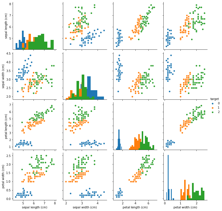
从上图可以发现,在2D情况下不同的特征组合对于不同类别的花的散点分布,以及大概的区分能力。
for col in iris_features.columns:
    sns.boxplot(x='target', y=col, saturation=0.5,
palette='pastel', data=iris_all)
    plt.title(col)
    plt.show()


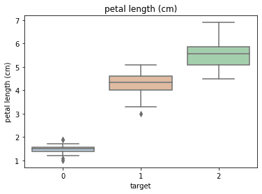

利用箱型图我们也可以得到不同类别在不同特征上的分布差异情况。
# 选取其前三个特征绘制三维散点图
from mpl_toolkits.mplot3d import Axes3D

fig = plt.figure(figsize=(10,8))
ax = fig.add_subplot(111, projection='3d')

iris_all_class0 = iris_all[iris_all['target']==0].values
iris_all_class1 = iris_all[iris_all['target']==1].values
iris_all_class2 = iris_all[iris_all['target']==2].values
# 'setosa'(0), 'versicolor'(1), 'virginica'(2)
ax.scatter(iris_all_class0[:,0], iris_all_class0[:,1], iris_all_class0[:,2],label='setosa')
ax.scatter(iris_all_class1[:,0], iris_all_class1[:,1], iris_all_class1[:,2],label='versicolor')
ax.scatter(iris_all_class2[:,0], iris_all_class2[:,1], iris_all_class2[:,2],label='virginica')
plt.legend()

plt.show()

Step5:利用 逻辑回归模型 在二分类上 进行训练和预测
##为了正确评估模型性能,将数据划分为训练集和测试集,并在训练集上训练模型,在测试集上验证模型性能。
from sklearn.model_selection import train_test_split
##选择其类别为0和1的样本(不包括类别为2的样本)
iris_features_part=iris_features.iloc[:100]
iris_target_part=iris_target[:100]
##测试集大小为20%,80%/20%分
x_train,x_test,y_train,y_test=train_test_split(iris_features_part,iris_target_part,test_size=0.2,random_state=2020)


##从sklearn中导入逻辑回归模型
from sklearn.linear_model import LogisticRegression

##定义逻辑回归模型
clf=LogisticRegression(random_state=0,solver='lbfgs')

##在训练集上训练逻辑回归模型
clf.fit(x_train,y_train)


##查看其对应的w
print('the weight of Logistic Regression:',clf.coef_)

##查看其对应的w0
print('the intercept(w0) of Logistic Regression:',clf.intercept_)


##在训练集和测试集上分布利用训练好的模型进行预测
train_predict=clf.predict(x_train)
test_predict=clf.predict(x_test)


from sklearn import metrics
##利用accuracy(准确度)【预测正确的样本数目占总预测样本数目的比例】评估模型效果
print('The accuracy of the Logistic Regression is:',metrics.accuracy_score(y_train,train_predict))
print('The accuracy of the Logistic Regression is:',metrics.accuracy_score(y_test,test_predict))

##查看混淆矩阵(预测值和真实值的各类情况统计矩阵)
confusion_matrix_result=metrics.confusion_matrix(test_predict,y_test)
print('The confusion matrix result:
',confusion_matrix_result)

##利用热力图对于结果进行可视化
plt.figure(figsize=(8,6))
sns.heatmap(confusion_matrix_result,annot=True,cmap='Blues')
plt.xlabel('Predictedlabels')
plt.ylabel('Truelabels')
plt.show()

##The accuracy of the Logistic Regressionis:1.0
##The accuracy of the Logistic Regressionis:1.0
##The confusion matrix result:
##[[9  0]
##[0  11]]
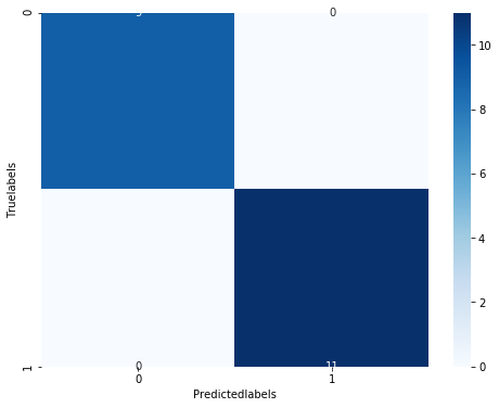
我们可以发现其准确度为1,代表所有的样本都预测正确了。
Step6:利用 逻辑回归模型 在三分类(多分类)上 进行训练和预测
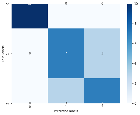
##测试集大小为20%,80%/20%分
x_train,x_test,y_train,y_test=train_test_split(iris_features,iris_target,test_size=0.2,random_state=2020)


##定义逻辑回归模型
clf=LogisticRegression(random_state=0,solver='lbfgs')


##在训练集上训练逻辑回归模型
clf.fit(x_train,y_train)


##查看其对应的w
print('the weight of Logistic Regression:
',clf.coef_)
##查看其对应的w0
print('the intercept(w0) of Logistic Regression:
',clf.intercept_)
##由于这个是3分类,所有我们这里得到了三个逻辑回归模型的参数,其三个逻辑回归组合起来即可实现三分类


##在训练集和测试集上分布利用训练好的模型进行预测
train_predict=clf.predict(x_train)
test_predict=clf.predict(x_test)
##由于逻辑回归模型是概率预测模型(前文介绍的p=p(y=1|x,	heta)),所有我们可以利用predict_proba函数预测其概率

train_predict_proba=clf.predict_proba(x_train)
test_predict_proba=clf.predict_proba(x_test)

print('The test predict Probability of each class:
',test_predict_proba)
##其中第一列代表预测为0类的概率,第二列代表预测为1类的概率,第三列代表预测为2类的概率。

##利用accuracy(准确度)【预测正确的样本数目占总预测样本数目的比例】评估模型效果
print('The accuracy of the Logistic Regression is:',metrics.accuracy_score(y_train,train_predict))
print('The accuracy of the Logistic Regression is:',metrics.accuracy_score(y_test,test_predict))


##查看混淆矩阵
confusion_matrix_result=metrics.confusion_matrix(test_predict,y_test)
print('The confusion matrix result:
',confusion_matrix_result)

##利用热力图对于结果进行可视化
plt.figure(figsize=(8,6))
sns.heatmap(confusion_matrix_result,annot=True,cmap='Blues')
plt.xlabel('Predicted labels')
plt.ylabel('True labels')
plt.show()

##The confusion matrix result:
##[[10  0   0]
##[0   8   2]
##[0   2   8]]
全部代码如下(已折叠):
# -*- coding: utf-8 -*-
"""
Created on Mon May 18 17:53:32 2020

@author: Admin
"""

#Step1:库函数导入
##  基础函数库
import numpy as np
import pandas as pd

## 绘图函数库
import matplotlib.pyplot as plt
import seaborn as sns


#SStep2:数据读取/载入
##我们利用sklearn中自带的iris数据作为数据载入,并利用Pandas转化为DataFrame格式
from sklearn.datasets import load_iris
data = load_iris() #得到数据特征
iris_target = data.target #得到数据对应的标签
iris_features = pd.DataFrame(data=data.data, columns=data.feature_names) #利用Pandas转化为DataFrame格式


#Step3:数据信息简单查看
##利用.info()查看数据的整体信息
iris_features.info()
'''
<class 'pandas.core.frame.DataFrame'>
RangeIndex: 150 entries, 0 to 149
Data columns (total 4 columns):
sepal length (cm)    150 non-null float64
sepal width (cm)     150 non-null float64
petal length (cm)    150 non-null float64
petal width (cm)     150 non-null float64
dtypes: float64(4)
memory usage: 4.8 KB
'''
##进行简单的数据查看,我们可以利用.head()头部.tail()尾部
iris_features.head()

'''
   sepal length (cm)  sepal width (cm)  petal length (cm)  petal width (cm)
0                5.1               3.5                1.4               0.2
1                4.9               3.0                1.4               0.2
2                4.7               3.2                1.3               0.2
3                4.6               3.1                1.5               0.2
4                5.0               3.6                1.4               0.2

'''

iris_features.tail()

'''
  sepal length (cm)  sepal width (cm)  petal length (cm)  petal width (cm)
145                6.7               3.0                5.2               2.3
146                6.3               2.5                5.0               1.9
147                6.5               3.0                5.2               2.0
148                6.2               3.4                5.4               2.3
149                5.9               3.0                5.1               1.8

'''
##其对应的类别标签为,其中0,1,2分别代表'setosa','versicolor','virginica'三种不同花的类别

iris_target
'''
array([0, 0, 0, 0, 0, 0, 0, 0, 0, 0, 0, 0, 0, 0, 0, 0, 0, 0, 0, 0, 0, 0,
       0, 0, 0, 0, 0, 0, 0, 0, 0, 0, 0, 0, 0, 0, 0, 0, 0, 0, 0, 0, 0, 0,
       0, 0, 0, 0, 0, 0, 1, 1, 1, 1, 1, 1, 1, 1, 1, 1, 1, 1, 1, 1, 1, 1,
       1, 1, 1, 1, 1, 1, 1, 1, 1, 1, 1, 1, 1, 1, 1, 1, 1, 1, 1, 1, 1, 1,
       1, 1, 1, 1, 1, 1, 1, 1, 1, 1, 1, 1, 2, 2, 2, 2, 2, 2, 2, 2, 2, 2,
       2, 2, 2, 2, 2, 2, 2, 2, 2, 2, 2, 2, 2, 2, 2, 2, 2, 2, 2, 2, 2, 2,
       2, 2, 2, 2, 2, 2, 2, 2, 2, 2, 2, 2, 2, 2, 2, 2, 2, 2])

'''
##利用value_counts函数查看每个类别数量

pd.Series(iris_target).value_counts()

##2    50

##1    50

##0    50

##dtype:int64

##对于特征进行一些统计描述

iris_features.describe()

'''
      sepal length (cm)  sepal width (cm)  petal length (cm)  petal width (cm)
count         150.000000        150.000000         150.000000        150.000000
mean            5.843333          3.057333           3.758000          1.199333
std             0.828066          0.435866           1.765298          0.762238
min             4.300000          2.000000           1.000000          0.100000
25%             5.100000          2.800000           1.600000          0.300000
50%             5.800000          3.000000           4.350000          1.300000
75%             6.400000          3.300000           5.100000          1.800000
max             7.900000          4.400000           6.900000          2.500000

'''


#Step4:可视化描述
## 合并标签和特征信息
iris_all = iris_features.copy() ##进行浅拷贝,防止对于原始数据的修改
iris_all['target'] = iris_target

## 特征与标签组合的散点可视化
sns.pairplot(data=iris_all,diag_kind='hist', hue= 'target')
plt.show()


for col in iris_features.columns:
    sns.boxplot(x='target', y=col, saturation=0.5,
palette='pastel', data=iris_all)
    plt.title(col)
    plt.show()


 # 选取其前三个特征绘制三维散点图
from mpl_toolkits.mplot3d import Axes3D

fig = plt.figure(figsize=(10,8))
ax = fig.add_subplot(111, projection='3d')

iris_all_class0 = iris_all[iris_all['target']==0].values
iris_all_class1 = iris_all[iris_all['target']==1].values
iris_all_class2 = iris_all[iris_all['target']==2].values
# 'setosa'(0), 'versicolor'(1), 'virginica'(2)
ax.scatter(iris_all_class0[:,0], iris_all_class0[:,1], iris_all_class0[:,2],label='setosa')
ax.scatter(iris_all_class1[:,0], iris_all_class1[:,1], iris_all_class1[:,2],label='versicolor')
ax.scatter(iris_all_class2[:,0], iris_all_class2[:,1], iris_all_class2[:,2],label='virginica')
plt.legend()

plt.show()


# Step5:利用 逻辑回归模型 在二分类上 进行训练和预测
##为了正确评估模型性能,将数据划分为训练集和测试集,并在训练集上训练模型,在测试集上验证模型性能。
from sklearn.model_selection import train_test_split
##选择其类别为0和1的样本(不包括类别为2的样本)
iris_features_part=iris_features.iloc[:100]
iris_target_part=iris_target[:100]
##测试集大小为20%,80%/20%分
x_train,x_test,y_train,y_test=train_test_split(iris_features_part,iris_target_part,test_size=0.2,random_state=2020)


##从sklearn中导入逻辑回归模型
from sklearn.linear_model import LogisticRegression

##定义逻辑回归模型
clf=LogisticRegression(random_state=0,solver='lbfgs')

##在训练集上训练逻辑回归模型
clf.fit(x_train,y_train)


##查看其对应的w
print('the weight of Logistic Regression:',clf.coef_)

##查看其对应的w0
print('the intercept(w0) of Logistic Regression:',clf.intercept_)


##在训练集和测试集上分布利用训练好的模型进行预测
train_predict=clf.predict(x_train)
test_predict=clf.predict(x_test)


from sklearn import metrics
##利用accuracy(准确度)【预测正确的样本数目占总预测样本数目的比例】评估模型效果
print('The accuracy of the Logistic Regression is:',metrics.accuracy_score(y_train,train_predict))
print('The accuracy of the Logistic Regression is:',metrics.accuracy_score(y_test,test_predict))

##查看混淆矩阵(预测值和真实值的各类情况统计矩阵)
confusion_matrix_result=metrics.confusion_matrix(test_predict,y_test)
print('The confusion matrix result:
',confusion_matrix_result)

##利用热力图对于结果进行可视化
plt.figure(figsize=(8,6))
sns.heatmap(confusion_matrix_result,annot=True,cmap='Blues')
plt.xlabel('Predictedlabels')
plt.ylabel('Truelabels')
plt.show()

##The accuracy of the Logistic Regressionis:1.0
##The accuracy of the Logistic Regressionis:1.0
##The confusion matrix result:
##[[9  0]
##[0  11]]


#Step6:利用 逻辑回归模型 在三分类(多分类)上 进行训练和预测
##测试集大小为20%,80%/20%分
x_train,x_test,y_train,y_test=train_test_split(iris_features,iris_target,test_size=0.2,random_state=2020)


##定义逻辑回归模型
clf=LogisticRegression(random_state=0,solver='lbfgs')


##在训练集上训练逻辑回归模型
clf.fit(x_train,y_train)


##查看其对应的w
print('the weight of Logistic Regression:
',clf.coef_)
##查看其对应的w0
print('the intercept(w0) of Logistic Regression:
',clf.intercept_)
##由于这个是3分类,所有我们这里得到了三个逻辑回归模型的参数,其三个逻辑回归组合起来即可实现三分类


##在训练集和测试集上分布利用训练好的模型进行预测
train_predict=clf.predict(x_train)
test_predict=clf.predict(x_test)
##由于逻辑回归模型是概率预测模型(前文介绍的p=p(y=1|x,	heta)),所有我们可以利用predict_proba函数预测其概率

train_predict_proba=clf.predict_proba(x_train)
test_predict_proba=clf.predict_proba(x_test)

print('The test predict Probability of each class:
',test_predict_proba)
##其中第一列代表预测为0类的概率,第二列代表预测为1类的概率,第三列代表预测为2类的概率。

##利用accuracy(准确度)【预测正确的样本数目占总预测样本数目的比例】评估模型效果
print('The accuracy of the Logistic Regression is:',metrics.accuracy_score(y_train,train_predict))
print('The accuracy of the Logistic Regression is:',metrics.accuracy_score(y_test,test_predict))


##查看混淆矩阵
confusion_matrix_result=metrics.confusion_matrix(test_predict,y_test)
print('The confusion matrix result:
',confusion_matrix_result)

##利用热力图对于结果进行可视化
plt.figure(figsize=(8,6))
sns.heatmap(confusion_matrix_result,annot=True,cmap='Blues')
plt.xlabel('Predicted labels')
plt.ylabel('True labels')
plt.show()

##The confusion matrix result:
##[[10  0   0]
##[0   8   2]
##[0   2   8]]
逻辑回归原理简介
当z≥0 时,y≥0.5,分类为1,当 z<0时,y<0.5,分类为0,其对应的y值我们可以视为类别1的概率预测值。Logistic回归虽然名字里带“回归”,但是它实际上是一种分类方法,主要用于两分类问题(即输出只有两种,分别代表两个类别),所以利用了Logistic函数(或称为Sigmoid函数),函数形式为:
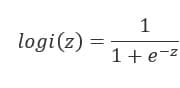
对应的函数图像可以表示如下:
import numpy as np
import matplotlib.pyplot as plt
x = np.arange(-5,5,0.01)
y = 1/(1+np.exp(-x))

plt.plot(x,y)
plt.xlabel('z')
plt.ylabel('y')
plt.grid()
plt.show()
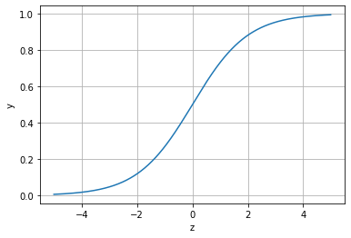
通过上图我们可以发现 Logistic 函数是单调递增函数,并且在z=0,而回归的基本方程,将回归方程写入其中为:
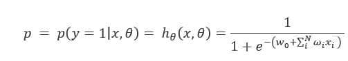

所以,逻辑回归从其原理上来说,逻辑回归其实是实现了一个决策边界:对于函数 ,当z≥0 时,y≥0.5,分类为1,当 z<0时,y<0.5,分类为0,其对应的y值我们可以视为类别1的概率预测值。
对于模型的训练而言:实质上来说就是利用数据求解出对应的模型的特定的ω。从而得到一个针对于当前数据的特征逻辑回归模型。而对于多分类而言,将多个二分类的逻辑回归组合,即可实现多分类。
群里面有优秀的同学的回答:
首先逻辑回归的基础是线性回归,通过一个线性方程将输入的特征值输出为预测值y,但是y的取值范围是正无穷到负无穷,并不是0或1,
因而逻辑回归通过一个函数来归一化y值,使y的取值在区间(0,1)内,这个函数就是logistic函数,也就是我们通常说的sigmoid函数,它只是sigmoid函数的一种;
logistic函数的优点:
    1.logistic函数可以压缩数据,不管x取什么值,对应的函数值总是在(0,1)范围内;
    2.logistic函数和其反函数都是严格单调递增的;
    3.logistic函数连续、光滑,易于求导;
    4.logistic函数关于点(0, 0.5)对称。
缺点:
    1.在趋向无穷的地方,函数值变化很小,容易缺失梯度。