0. 才话别已深秋
今天我可能要当搬运工了,我看这本书的最后一点内容让我觉得....有所收获和反思。然后我发现每一本机器学习书和教材一定会有“用TF怎么实现无监督的迭代聚类算法”,而且一定会放在最后一章节Tensorflow的进阶应用里面。不夸张的说,KNN、Kmeans、贝叶斯分类,这三个算法是当时大二下刘建毅课上接触到的。当时大作业是切词分词+文本分类任务,我们用的贝叶斯算法分类。所以其实是很古老很古老的东西了,不知道为什么要算作进阶....
其实还有一些原因促使我想要更新这一篇吧。第一个,我之前投的那篇论文其实就是基于分布式系统的文摘算法,中间步骤的聚类还是特么用的Canopy-Kmeans。第二个,上周打大数据比赛的时候,我们想对用户人群做聚类。但当时我们是想按照两个特征的余弦距离判别相似性的,但是但是,特么的K-means里面用余弦相似会出现奇怪的错误!或者说聚类结果需要花很大很大功夫去做数据分析,当时给我们添了不少堵啊。而且在聚完类做降维画图分析的时候,也是遇到巨大的问题真的。平时没遇到的问题,去网上临时抱佛脚看得真的很累。我们当时特征降维绘图用的t-sne,完全不知道原理好吧。我今天看到这个我才知道降维的还有PAC和SVD,稍微也看了下原理。贴一篇PAC降维的参考,基于主成分分析的,也就是奇异矩阵分解:https://www.cnblogs.com/NextNight/p/6180542.html。
下次有空在更新吧。
小黑喵施工 ing....
1. 只一眼
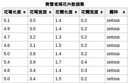
数据集为iris,是一个给花做分类的数据集。相信很多学习分类算法或者sklearn库都很熟悉这个东西。每个样本包含了花的花萼长度、宽度,花瓣长度、花瓣宽度四个特征,最后再加上一个label。所以每个样本就1行5列。大概长相如下,然后现在不需要单独下载,数据集封装在python sklearn里面。
然后是代码。代码参考书上的k-means部分,然后修改了一些编译错误的地方,跟之前一样的环境可以直接运行。
|
# -*- coding: utf-8 -*-
# # Tensorflow下的Kmeans算法 # 使用sklearn库中的iris数据集对三种花进行聚类 # 利用PCA分解进行降维展示 # # 参考:《Tensorflow机器学习实战指南》第11章第5节 #---------------------------------- # import numpy as np import matplotlib.pyplot as plt import tensorflow as tf from sklearn import datasets from scipy.spatial import cKDTree from sklearn.decomposition import PCA from sklearn.preprocessing import scale from tensorflow.python.framework import ops ops.reset_default_graph() # 创建计算图会话。加载iris数据集 sess = tf.Session() iris = datasets.load_iris() num_pts = len(iris.data) num_feats = len(iris.data[0]) # 设置K值为3。iris数据集有三类花 # 实际上是分类任务,因为已经给了堆大小了 # 迭代次数25 k=3 generations = 25 # 计算图参数 data_points = tf.Variable(iris.data) cluster_labels = tf.Variable(tf.zeros([num_pts], dtype=tf.int64)) # 先随机选择iris数据集中的三个数据点作为每个堆的中心点 rand_starts = np.array([iris.data[np.random.choice(len(iris.data))] for _ in range(k)]) centroids = tf.Variable(rand_starts) # 计算每个数据点到每个中心点的欧氏距离 # 这里是将数据点都放入矩阵,直接按矩阵进行运算 centroid_matrix = tf.reshape(tf.tile(centroids, [num_pts, 1]), [num_pts, k, num_feats]) point_matrix = tf.reshape(tf.tile(data_points, [1, k]), [num_pts, k, num_feats]) distances = tf.reduce_sum(tf.square(point_matrix - centroid_matrix), axis=2) # 分配时,以每个数据点最小距离为最接近的中心点 centroid_group = tf.argmin(distances, 1) # 计算三个堆的平均距离更新堆中新的中心点 def data_group_avg(group_ids, data): # 分组求和 sum_total = tf.unsorted_segment_sum(data, group_ids, 3) # 计算堆大小 num_total = tf.unsorted_segment_sum(tf.ones_like(data), group_ids, 3) # 求距离均值 avg_by_group = sum_total/num_total return(avg_by_group) means = data_group_avg(centroid_group, data_points) update = tf.group(centroids.assign(means), cluster_labels.assign(centroid_group)) # 初始化模型变量 init = tf.global_variables_initializer() sess.run(init) # 遍历循环训练,更新每组分类的中心点 for i in range(generations): print('Calculating gen {}, out of {}.'.format(i, generations)) _, centroid_group_count = sess.run([update, centroid_group]) group_count = [] for ix in range(k): group_count.append(np.sum(centroid_group_count==ix)) print('Group counts: {}'.format(group_count)) # 输出准确率。 # 聚类结果和iris数据集中的标签进行对比 [centers, assignments] = sess.run([centroids, cluster_labels]) def most_common(my_list): return(max(set(my_list), key=my_list.count)) label0 = most_common(list(assignments[0:50])) label1 = most_common(list(assignments[50:100])) label2 = most_common(list(assignments[100:150])) group0_count = np.sum(assignments[0:50]==label0) group1_count = np.sum(assignments[50:100]==label1) group2_count = np.sum(assignments[100:150]==label2) accuracy = (group0_count + group1_count + group2_count)/150. print('Accuracy: {:.2}'.format(accuracy)) # 可视化部分 # 使用降维分解工具PCA # 将数据由4维降至2维可作图 pca_model = PCA(n_components=2) reduced_data = pca_model.fit_transform(iris.data) reduced_centers = pca_model.transform(centers) # 设置绘图的mersh大小 h = .02 # 设置背景颜色 x_min, x_max = reduced_data[:, 0].min() - 1, reduced_data[:, 0].max() + 1 y_min, y_max = reduced_data[:, 1].min() - 1, reduced_data[:, 1].max() + 1 xx, yy = np.meshgrid(np.arange(x_min, x_max, h), np.arange(y_min, y_max, h)) # 根据分类设置grid point颜色 xx_pt = list(xx.ravel()) yy_pt = list(yy.ravel()) xy_pts = np.array([[x,y] for x,y in zip(xx_pt, yy_pt)]) mytree = cKDTree(reduced_centers) dist, indexes = mytree.query(xy_pts) indexes = indexes.reshape(xx.shape) plt.figure(1) plt.clf() plt.imshow(indexes, interpolation='nearest', extent=(xx.min(), xx.max(), yy.min(), yy.max()), cmap=plt.cm.Paired, aspect='auto', origin='lower') # 设置图例 symbols = ['o', '^', 'D'] label_name = ['Setosa', 'Versicolour', 'Virginica'] for i in range(3): temp_group = reduced_data[(i*50):(50)*(i+1)] plt.plot(temp_group[:, 0], temp_group[:, 1], symbols[i], markersize=10, label=label_name[i]) # 绘图 plt.scatter(reduced_centers[:, 0], reduced_centers[:, 1], marker='x', s=169, linewidths=3, color='w', zorder=10) plt.title('K-means clustering on Iris Dataset ' 'Centroids are marked with white cross') plt.xlim(x_min, x_max) plt.ylim(y_min, y_max) plt.legend(loc='lower right') plt.show() |
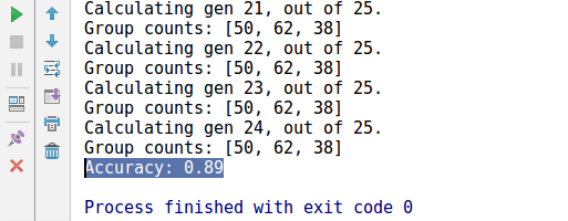
运行效果和绘图如下:

2. 花落
最后用K-means预测的类标和真实类标相比达到了89%的准确率。主要是上图中右侧两种类型花的非线性分类关系是K-means很难学习到的,解决这个问题的话使用SVM加强非线性分类可能会好一点。不过写这篇博文还真不是为了学K-means什么的,毕竟用别人的不就好了吗,而且何必要用TF来实现呢。只是做数据竞赛啊之类的,聚类分类降维这些基本手段真的太重要了。不吃点亏还真不知道有多严重,书到用时方恨少啊。既然想起了,那就安安静静听听歌记录下来吧。