1. 读取数据集
def load_data(filename,dataType):
    return np.loadtxt(filename,delimiter=",",dtype = dataType)

def read_data():
    data = load_data("data2.txt",np.float64)
    X = data[:,0:-1]
    y = data[:,-1]
    return X,y
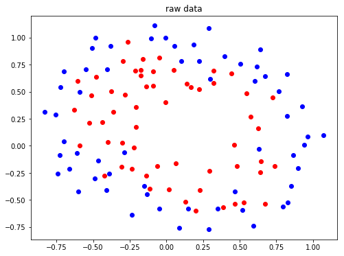
2. 查看原始数据的分布
def plot_data(x,y):
    pos = np.where(y==1) # 找到标签为1的位置
    neg = np.where(y==0) #找到标签为0的位置

    plt.figure(figsize=(8,6))
    plt.plot(x[pos,0],x[pos,1],'ro')
    plt.plot(x[neg,0],x[neg,1],'bo')
    plt.title("raw data")
    plt.show()

X,y = read_data()
plot_data(X,y)
结果:
3. 将数据映射为多项式
由原图数据分布可知,数据的分布是非线性的,这里将数据变为多项式的形式,使其变得可分类。
映射为二次方的形式:
def mapFeature(x1,x2):
    degree = 2;   #映射的最高次方
    out = np.ones((x1.shape[0],1)) # 映射后的结果数组(取代X)

    for i in np.arange(1,degree+1):
        for j in range(i+1):
            temp = x1 ** (i-j) * (x2**j)
            out = np.hstack((out,temp.reshape(-1,1)))
    return out
4. 定义交叉熵损失函数
可以综合起来为:
其中:
为了防止过拟合,加入正则化技术:
注意j是重1开始的,因为theta(0)为一个常数项,X中最前面一列会加上1列1,所以乘积还是theta(0),feature没有关系,没有必要正则化
def sigmoid(x):
    return 1.0 / (1.0+np.exp(-x))

def CrossEntropy_loss(initial_theta,X,y,inital_lambda):   #定义交叉熵损失函数
    m = len(y)
    h = sigmoid(np.dot(X,initial_theta))
    theta1 = initial_theta.copy()           # 因为正则化j=1从1开始,不包含0,所以复制一份,前theta(0)值为0
    theta1[0] = 0

    temp = np.dot(np.transpose(theta1),theta1)
    loss = (-np.dot(np.transpose(y),np.log(h)) - np.dot(np.transpose(1-y),np.log(1-h)) + temp*inital_lambda/2) / m
    return loss
5. 计算梯度
对上述的交叉熵损失函数求偏导:
利用梯度下降法进行优化:
def gradientDescent(initial_theta,X,y,initial_lambda,lr,num_iters):
    m = len(y)

    theta1 = initial_theta.copy()
    theta1[0] = 0
    J_history = np.zeros((num_iters,1))

    for i in range(num_iters):
        h = sigmoid(np.dot(X,theta1))
        grad = np.dot(np.transpose(X),h-y)/m + initial_lambda * theta1/m
        theta1 = theta1 - lr*grad
        #print(theta1)
        J_history[i] = CrossEntropy_loss(theta1,X,y,initial_lambda)
    return theta1,J_history
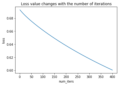
6. 绘制损失值随迭代次数的变化曲线
def plotLoss(J_history,num_iters):
    x = np.arange(1,num_iters+1)
    plt.plot(x,J_history)
    plt.xlabel("num_iters")
    plt.ylabel("loss")
    plt.title("Loss value changes with the number of iterations")
    plt.show()
7. 绘制决策边界
def plotDecisionBoundary(theta,x,y):
    pos = np.where(y==1)  #找到标签为1的位置
    neg = np.where(y==0)  #找到标签为2的位置

    plt.figure(figsize=(8,6))
    plt.plot(x[pos,0],x[pos,1],'ro')
    plt.plot(x[neg,0],x[neg,1],'bo')
    plt.title("Decision Boundary")

    #生成和原数据类似的数据
    u = np.linspace(-1,1.5,50)
    v = np.linspace(-1,1.5,50)
    z = np.zeros((len(u),len(v)))
    #利用训练好的参数做预测
    for i in range(len(u)):
        for j in range(len(v)):
            z[i,j] = np.dot(mapFeature(u[i].reshape(1,-1),v[j].reshape(1,-1)),theta)

    z = np.transpose(z)
    plt.contour(u,v,z,[0,0.01],linewidth=2.0)   # 画等高线,范围在[0,0.01],即近似为决策边界
    plt.legend()
    plt.show()
8.主函数
if __name__ == "__main__":

    #数据的加载
    x,y = read_data()
    X = mapFeature(x[:,0],x[:,1])
    Y = y.reshape((-1,1))

    #参数的初始化
    num_iters = 400
    lr = 0.1
    initial_theta = np.zeros((X.shape[1],1))  #初始化参数theta
    initial_lambda = 0.1 #初始化正则化系数

    #迭代优化
    theta,loss = gradientDescent(initial_theta,X,Y,initial_lambda,lr,num_iters)
    plotLoss(loss,num_iters)
    plotDecisionBoundary(theta,x,y)
9.结果