本代码参考自:https://github.com/lawlite19/MachineLearning_Python#%E4%B8%80%E7%BA%BF%E6%80%A7%E5%9B%9E%E5%BD%92
首先,线性回归公式:y = X*W +b 其中X是m行n列的数据集,m代表样本的个数,n代表每个样本的数据维度。则W是n行1列的数据,b是m行1列的数据,y也是。
损失函数采用MSE,采用梯度下降法进行训练
1 .加载数据集并进行读取
def load_csvdata(filename,split,dataType):        #加载数据集
    return np.loadtxt(filename,delimiter = split,dtype = dataType)

def read_data():  #读取数据集
    data = load_csvdata("data.txt",split=",",dataType=np.float64)
    print(data.shape)
    X = data[:,0:-1] #取data的前两列
    y = data[:,-1]   #取data的最后一列作为标签
    return X,y
2 . 对数据进行标准化
def feature_normalization(X):
    X_norm = np.array(X)
    mu = np.zeros((1,X.shape[1]))
    std = np.zeros((1,X.shape[1]))
    mu = np.mean(X_norm,0)
    std = np.std(X_norm,0)
    for i in range(X.shape[1]):
        X_norm[:,i] = (X_norm[:,i] - mu[i]) / std[i]
    return X_norm,mu,std
3. 损失值的计算
def loss(X,y,w):
    m = len(y)
    J = 0
    J = (np.transpose(X*w - y))*(X*w - y) / (2*m)
    print(J)
    return J
4. 梯度下降算法的python实现
def gradientDescent(X,y,w,lr,num_iters):
    m = len(y)  #获取数据集长度
    n = len(w)  #获取每个输入数据的维度
    temp = np.matrix(np.zeros((n,num_iters)))
    J_history = np.zeros((num_iters,1))
    for i in range(num_iters): #进行迭代
        h = np.dot(X,w)   #线性回归的矢量表达式
        temp[:,i] = w - ((lr/m)*(np.dot(np.transpose(X),h-y))) #梯度的计算
        w = temp[:,i]
        J_history[i] = loss(X,y,w)
    return w,J_history
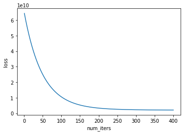
5. 绘制损失值随迭代次数变化的曲线图
def plotLoss(J_history,num_iters):
    x = np.arange(1,num_iters+1)
    plt.plot(x,J_history)
    plt.xlabel("num_iters")
    plt.ylabel("loss")
    plt.title("Loss value changes with the number of iterations")
    plt.show()
6. 主函数
if __name__ == "__main__":
    X,y = read_data()
    X,mu,sigma = feature_normalization(X)
    m = len(y)     #样本的总个数
    X = np.hstack((np.ones((m,1)),X))   #在x上加上1列是为了计算偏移b   X=[x0,x1,x2,......xm] 其中x0=1 y = x*w
    y = y.reshape((-1,1))
    lr = 0.01
    num_iters = 400
    w = np.random.normal(scale=0.01, size=((X.shape[1],1)))
    theta,J_history = gradientDescent(X,y,w,lr,num_iters)
    plotLoss(J_history,num_iters)
7.结果