Ch12 Resampling statistics and bootstrapping
Permutation tests
Permutation tests, also called randomization or re-randomization tests.
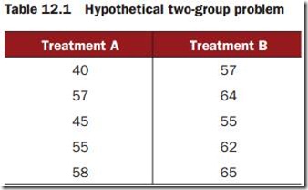
Ten subjects have been randomlyassigned to one of two treatment conditions(A or B) and an outcome variable (score) has been recorded.
Is there enough evidence to conclude that the treatments differ in their impact?
In a parametric approach, you might assume that the data are sampled from normal populations with equal variances and apply a two-tailed independent groups t-test. The null hypothesis is that the population mean for treatment A is equal to the population mean for treatment B.
A permutation test takes a different approach. If the two treatments are truly quivalent, the label (Treatment A or Treatment B) assigned to an observed score is arbitrary.
To test for differences between the two treatments, we could follow these steps:
1 Calculate the observed t-statistic, as in the parametric approach; call this t0.
2 Place all 10 scores in a single group.
3 Randomly assign five scores to Treatment A and five scores to Treatment B.
4 Calculate and record the new observed t-statistic.
5 Repeat steps 3–4 for every possible way of assigning five scores to Treatment A and five scores to Treatment B. There are 252 such possible arrangements.
6 Arrange the 252 t-statistics in ascending order. This is the empirical distribution, based on (or conditioned on) the sample data.
7 If t0 falls outside the middle 95 percent of the empirical distribution, reject the null hypothesis that the population means for the two treatment groups are equal at the 0.05 level of significance.
install.packages(c(“coin”,"lmPerm"))
The coin package provides a comprehensive framework for permutation tests applied to independence problems, whereas the lmPerm package provides permutation tests for ANOVA and regression designs.
Permutation test with the coin package
Applying permutation tests to independence problems.
Are responses independent of group assignment?
Are two categorical variables independent?
Are two numeric variables independent?
function_name( formula, data, distribution= )
formula describes the relationship among variables to be tested.
data identifies a data frame.
distribution specifies how the empirical distribution under the null hypothesis should be derived. Possible values are exact, asymptotic, and approximate.
Independent two-sample and k-sample tests
t-test versus one-way per mutation test for the hypothetical data
library(coin)
score <- c(40, 57, 45, 55, 58, 57, 64, 55, 62, 65)
treatment <- factor(c(rep("A",5), rep("B",5)))
mydata <- data.frame(treatment, score)
t.test(score~treatment, data=mydata, var.equal=TRUE)
oneway_test(score~treatment, data=mydata, distribution="exact")
eg2:
library(MASS)
UScrime <- transform(UScrime, So = factor(So))
wilcox_test(Prob ~ So, data=UScrime, distribution="exact")
The numeric variable So was transformed into a factor. This is because the coin package requires that all categorical variables be coded as factors.
Finally, consider a k-sample test.
In chapter 9, we used a one-way ANOVA to evaluate the impact of five drug regimens on cholesterol reduction in a sample of 50 patients. An approximate k-sample permutation test can be per formed instead:
library(multcomp)
set.seed(1234)
oneway_test(response~trt, data=cholesterol, distribution=approximate(B=9999))
12.2.2 Independence in contingency tables
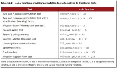
We can use permutation tests to assess the independence of two categorical variables using either thechisq_test() or the cmh_test() function. The latter function is used when the data is stratified on a third categorical variable. If both variables are ordinal, we can use the lbl_test() function to test for a linear trend.
library(coin)
library(vcd)
Arthritis <- transform(Arthritis, Improved=as.factor(as.numeric(Improved)))
set.seed(1234)
chisq_test(Treatment~Improved, data=Arthritis,distribution=approximate(B=9999))
You might ask why you transformed the variable Improved from an ordered factor to a categorical factor. (Good question!) If you’d left it an ordered factor, coin() would have generated a linear x linear trend test instead of a chi-square test.
12.2.3 Independence between numeric variables
The spearman_test() function provides a permutation test of the independence of two numeric variables.
states <- as.data.frame(state.x77)
set.seed(1234)
spearman_test(Illiteracy~Murder, data=states, distribution=approximate(B=9999))
12.2.4 Dependent two-sample and k-sample tests
Dependent sample tests are used when obser vations in different groups have been matched, or when repeated measures are used. For permutation tests with two paired groups, the wilcoxsign_test() function can be used. For more than two groups, use the friedman_test() function.
library(coin)
library(MASS)
wilcoxsign_test(U1~U2, data=UScrime, distribution="exact")
12.2.5 Going further
The coin package provides a general framework for testing that one group of variables is independent of a second group of variables (with optional stratification on a blocking variable) against arbitrary alternatives, via approximate permutation tests.
In particular, the independence_test() function allows the user to approach most traditional tests from a permutation perspective, and to create new and novel statistical tests for situations not covered by traditional methods. This flexibility comes at a price: a high level of statistical knowledge is required to use the function appropriately. See the vignettes that accompany the package (accessed via vignette("coin")) for further details.
12.3 Permutation tests with the lmPerm package
The lmPerm package provides support for a permutation approach to linear models, including regression and analysis of variance. The lmp() and aovp() functions are the lm() and aov() functions modified to per form permutation tests rather than normal theory tests.
12.3.1 Simple and polynomial regression
Listing 12.2 Permutation tests for simple linear regression
library(lmPerm)
set.seed(1234)
fit <- lmp(weight~height, data=women, perm="Prob")
Listing 12.3 Permutation tests for polynomial regression
library(lmPerm)
set.seed(1234)
fit <- lmp(weight~height + I(height^2), data=women, perm="Prob")
12.3.2 Multiple regression
Listing 12.4 Permutation tests for multiple regression
library(lmPerm)
set.seed(1234)
states <- as.data.frame(state.x77)
fit <- lmp(Murder~Population + Illiteracy+Income+Frost,data=states, perm="Prob")
12.3.3 One-way ANOVA and ANCOVA
Listing 12.5 Permutation test for One-Way ANOVA
library(lmPerm)
library(multcomp)
set.seed(1234)
fit <- aovp(response~trt, data=cholesterol, perm="Prob")
Listing 12.6 Permutation test for one-way ANCOVA
library(lmPerm)
set.seed(1234)
fit <- aovp(weight ~ gesttime + dose, data=litter, perm="Prob")
12.3.4 Two-way ANOVA
Listing 12.7 Permutation test for two-way ANOVA
library(lmPerm)
set.seed(1234)
fit <- aovp(len~supp*dose, data=ToothGrowth, perm="Prob")
12.4 Additional comments on permutation tests
The corrperm package provides permutation tests of correlations with repeated measures.
The logregperm package offers a permutation test for logistic regression.
The glmperm package extends permutation tests to generalized linear models.
Permutation tests provide a powerful alternative to tests that rely on a knowledge of the underlying sampling distribution. In each of the permutation tests described, we were able to test statistical hypotheses without recourse to the normal, t, F, or chi-square distributions.
Where permutation tests really shine are in cases where the data is clearly non-normal (for example, highly skewed), outliers are present, samples sizes are small, or no parametric tests exist. However, if the original sample is a poor representation of the population of interest, no test, including permutation tests, will improve the inferences generated.
Permutation tests are primarily useful for generating p-values that can be used to test null hypotheses. They can help answer the question, “Does an effect exist?” It’s more difficult to use permutation methods to obtain confidence intervals and estimates of measurement precision.
12.5 Bootstrapping
Bootstrapping generates an empirical distribution of a test statistic or set of test statistics, by repeated random sampling with replacement, from the original sample. It allows you to generate confidence inter vals and test statistical hypotheses without having to assume a specific underlying theoretical distribution.
Your sample has 10 observations, a sample mean of 40, and a sample standard deviation of 5. If you’re willing to assume that the sampling distribution of the mean is normally distributed, the (1-α /2 )% confidence inter val can be calculated using
You could use a bootstrapping approach instead:
1 Randomly select 10 observations from the sample, with replacement after each selection. Some obser vations may be selected more than once, and some may
not be selected at all.
2 Calculate and record the sample mean.
3 Repeat steps 1 and 2 a thousand times.
4 Order the 1,000 sample means from smallest to largest.
5 Find the sample means representing the 2.5th and 97.5th percentiles. In this case, its the 25th number from the bottom and top. These are your 95 percent confidence limits.
12.6 Bootstrapping with the boot package
The boot package provides extensive facilities for bootstrapping and related resampling methods. You can bootstrap a single statistic (for example, a median), or a vector of statistics (for example, a set of regression coefficients).
install.packages("boot")
In general, bootstrapping involves three main steps:
1 Write a function that returns the statistic or statistics of interest. If there is a single statistic (for example, a median), the function should return a number.
If there is a set of statistics (for example, a set of regression coefficients), the function should return a vector.
2 Process this function through the boot() function in order to generate R bootstrap replications of the statistic(s).
3 Use the boot.ci() function to obtain confidence intervals for the statistic(s) generated in step 2.
bootobject <- boot(data=, statistic=, R=, ...)
data A vector, matrix, or data frame.
statistic A function that produces the k statistics to be bootstrapped (k=1 if bootstrapping a single statistic). The function should include an indices parameter that the boot() function can use to select cases for each replication (see examples in the text).
R Number of bootstrap replicates.
... Additional parameters to be passed to the function that is used to produce statistic(s) of interest.
The boot() function calls the statistic function R times.
You can access these elements as bootobject$t0 and bootobject$t.
Once you generate the bootstrap samples, you can use print() and plot() to examine the results. If the results look reasonable, you can use the boot.ci() function
to obtain confidence intervals for the statistic(s).
12.6.1 Bootstrapping a single statistic
The first task is to write a function for obtaining the R-squared value:
rsq <- function(formula, data, indices) {
d <- data[indices,]
fit <- lm(formula, data=d)
return(summary(fit)$r.square)
}
The function returns the R-square value from a regression. The d <- data[indices,] statement is required for boot() to be able to select samples.
You can then draw a large number of bootstrap replications (say, 1,000) with the following code:
library(boot)
set.seed(1234)
results <- boot(data=mtcars, statistic=rsq, R=1000, formula=mpg~wt+disp)
The boot object can be printed using
> print(results)
>plot(results)
>boot.ci(results, type=c("perc", "bca"))
12.6.2 Bootstrapping several statistics
Let’s get confidence intervals for the three model regression coefficients.
First, create a function that returns the vector of regression coefficients:
bs <- function(formula, data, indices) {
d <- data[indices,]
fit <- lm(formula, data=d)
return(coef(fit))
}
Then use this function to bootstrap 1,000 replications:
library(boot)
set.seed(1234)
results <- boot(data=mtcars, statistic=bs,
R=1000, formula=mpg~wt+disp)
print(results)
plot(results, index=2)
boot.ci(results, type="bca", index=2)
boot.ci(results, type="bca", index=3)
It’s worth addressing two questions that come up often:
How large does the original sample need to be?
How many replications are needed?
There’s no simple answer to the first question. Some say that an original sample size of 20–30 is sufficient for good results, as long as the sample is representative of the popu-lation. Random sampling from the population of interest is the most trusted method for assuring the original sample’s representativeness. With regard to the second ques-tion, I find that 1,000 replications are more than adequate in most cases. Computer power is cheap and you can always increase the number of replications if desired.


