直方图均衡化算法可以自己得到一个转换函数,将输出图像具有近似的均匀分布。直方图均衡化是结果可预测且容易实现。但对于一些特殊的案例,直方图均衡化试图得到均匀直方图的方法并不能达到效果,这类情况下,往往需要指定输出图像直方图的具体分布,能够输出具有指定分布直方图的算法就是直方图匹配;
算法原理:
仍然用(r)和(z)表示连续灰度变量,(p_r(r))和(p_z(z))表示连续概率密度函数,(s)是一个随机变量,
(s = T(r) = int_{0}^{r} p_r(w)dw) (1)
随机变量(z)具有性质:
(G(z) = int_{0}^{z} p_z(t)dt = s) (2)
因此就有了,(G(z) = T(r)) 并且
(z = G^{-1}(s) = G^{-1} left[T(r) ight]) (3)
如果(G^{-1})存在,且满足条件:单值且单调递增,值域为[0,1],方程1~3就定义了一个输出指定直方图匹配的过程。从输入图像得到(s),从指定的直方图分布得到(z),再有方程3就有了从输入(r)到输出(s)的映射。
但问题是,在实际实践中很难获得(G^{-1})和(T(r))的解析式。比较幸运的是,在离散情况下,问题会变得简单,最终得到的是理想指定分布的近似。
离散环境下:
(s_k = T(r_k) = sum_{j=0}^{k} P_r(r_j) = sum_{j=0}^{k} frac{n_j}{n} qquad k =0,1,2,...L-1) (4)
(v_k = G(z_k) = sum_{i=0}^{k} p_z(z_j) = s_k qquad k = 0,1,2,3,...L-1.) (5)
(z_k = G^{-1}left[T(r_k) ight] qquad k = 0,1,2,3,...L-1) (6)
(z_k = G^{-1}(s_k))
方程(4)将像素点从(r)的灰度空间映射到了(s)的灰度空间,而方程(5)定义了一个直方图随机变量的转换函数,从(z)的灰度空间到s的空间。方程(6)是(5)的逆变换,得到了具有指定直方图分布的随机变量。
其实,通俗的讲,有三个灰度空间({r_j}),({s_j}),({z_j}), (j = 0,1,2,...L-1)的一维数组。映射就是完成这样的过程:指定下标查找;下标构成了一个查找表,对于灰度级j,(r_j)映射到(s_j),(s_j)映射到(z_j),(r_j)和(z_j)都是[0,L-]的灰度空间,(s)是[0,1]的空间。
图(1)阐明了这样的关系:
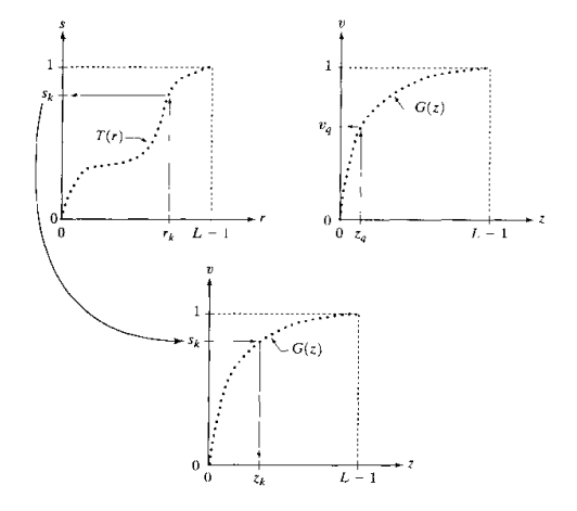
图(1)
左上角的图表示了一个假设的转换函数,对应于每一个(z_q),输出转换函数值(v_q),事实上我们需要的是这样的反过程,因为(v = s ),所以要找的就是为每一个(s_k),找到对应的(z_k)。
正因为(v = s),并且处理的是离散整型数据,所以寻找的(z_k)应该要满足条件(G(z_k) - s_k= 0),而由于(z)是一整数位步长的,所以要做的只是从小到大遍历(z_i),如果(z_i)是满足条件
(G(z_i)-s_k)ge 0) (7)
的最小整数,那么(z_k = z_i);
总结一下步骤:
(1):根据输入图像得到图像的灰度直方图(离散概率密度);
(2):根据方程(4)得到(s)
(3):由具有指定概率分布的随机变量(z)根据方程(5)得到G;
(4):以整数步长迭代(z),找到满足方程(7)的最小整数(z_i),即为对应(s_k)的(z_k)值;
实现:
MATLAB提供的histeq函数即可以做直方图均衡化,也可以做直方图匹配,只需将指定的概率密度函数作为参数传入即可。
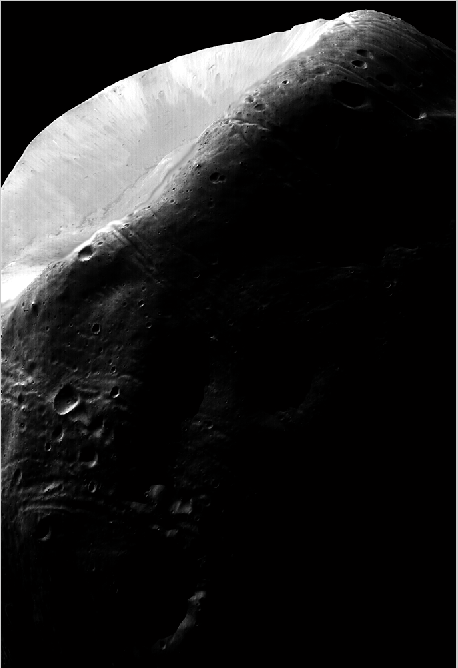
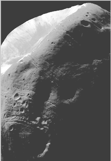
输入图像:
 1 >>f=imread('D:MATLABimageDIP3E_Original_Images_CH03Fig0323(a)(mars_moon_phobos).tif');
 2 >> hig = imhist(f);
 3 >> hig1 = hig(1:256);
 4 >> horz = 1:256;
 5 >> figure,stem(horz,hig1,'fill')
 6 >> axis([0 255 0 60000])
 7 >> set(gca,'xtick',[0:16:256])
 8 >> set(gca,'ytick',[0:6000:60000])
 9 >> figure,plot(horz,hig1,'color','b','linestyle','-','marker','.')
10 >> axis([0 255 0 60000])
11 >> set(gca,'xtick',[0:16:256])
12 >> set(gca,'ytick',[0:6000:60000])
 |
 |
 |
图(2)
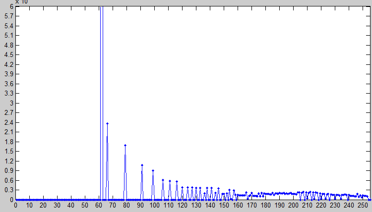
输入图像及其直方图,大部分像素点集中在较暗区域,直方图的左侧,如果对此做直方图均衡化,左边大量像素点将映射到较高的灰度区,并无法分散像素点,无法提高对比度。
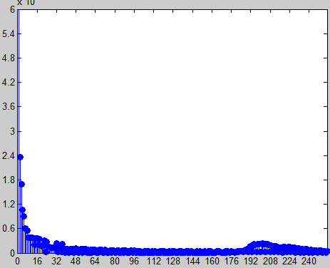
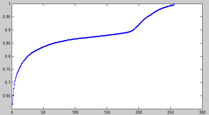
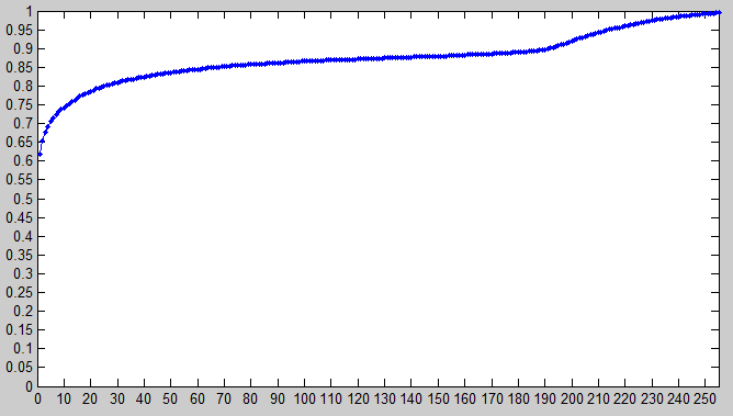
采用直方图匹配,首先要针对图像拟合一个可以提高对比度的输出图像的灰度概率分布函数,原图有两个峰值,将峰值出比较陡的灰度分布变为高斯分布,也许可以离散密集的灰度值,平缓峰值。可以根据方程(4)求得(s),s的函数图像为:
 |
 |
图(3)
拟合一个具有两个高斯峰值的输出函数,MATLAB代码:
 1 function p= twomodegauss( u1,sig1,u2,sig2,A1,A2,k)
 2 %bimodal gaussian function
 3 %   Detailed explanation goes here
 4 c1 = A1 *(1/((2*pi)^0.5)*sig1);
 5 c2 = A2 *(1/((2*pi)^0.5)*sig2);
 6 k1 = 2 * (sig1^2);
 7 k2 = 2 * (sig2^2);
 8 z = linspace(0,1,256);
 9 p = k + c1*exp(-((z-u1).^2)./k1)+c2 * exp(-((z-u2).^2)./k2);
10 p = p./sum(p(:));
11 end
 1 function p = manualhist
 2 %UNTITLED2 Summary of this function goes here
 3 %   Detailed explanation goes here
 4 flag = true;
 5 quitnow = 'x';
 6 p = twomodegauss(0.15,0.05,0.75,0.05,1,0.07,0.002);
 7 while flag
 8     s = input('enter m1,sig1,m2,sig2,A1,A2,k or x to quit:','s');
 9     if s== quitnow
10         break
11     end
12     v = str2num(s);
13     if numel(v) ~= 7
14         disp('incorret number of imputs')
15         continue
16     end
17     p  = twomodegauss(v(1),v(2),v(3),v(4),v(5),v(6),v(7));
18 end
19     figure,plot(p)
20     xlim([0 255])
21 end
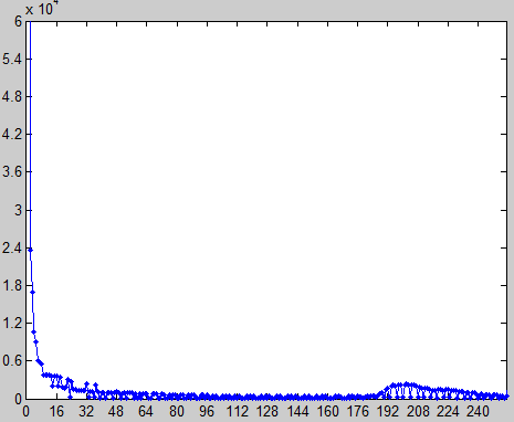
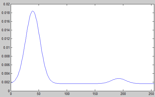
输出高斯函数及其CDF((G)):
 |
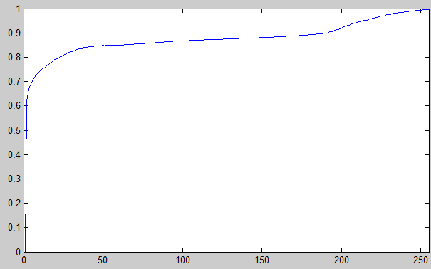 |
图(4)
输出图像要具有图(4)所示的灰度概率密度分布,需要完成直方图匹配过程,也就是方程(5)与步骤(4),MATLAB实现为histeq函数:
 1 >> g = histeq(f,p);
 2 >> imshow(g)
 3 Warning: Image is too big to fit on screen; displaying at 67%
 4 > In imuitoolsprivateinitSize at 73
 5   In imshow at 262
 6 >> hg = imhist(g);
 7 >> hg1 = hg(1:256);
 8 >> horz = 1:256;
 9 >> plot(horz,hg1,'color','b','linestyle','-','marker','.');
10 >> axis([0 255 0 60000])
11 >> set(gca,'xtick',[0:10:256])
12 >> set(gca,'ytick',[0:3000:60000])
输出效果图像:
 |
 |
图(5)
实现直方图匹配的C++算法:
 1 #define A1 1
 2 #define A2 0.07
 3 #define U1 0.15
 4 #define SIG1 0.05
 5 #define U2 0.75
 6 #define SIG2 0.05
 7 #define pi 3.1415626535627
 8 using namespace cimg_library;
 9
10 inline float twoModeGauss(float r){
11     //double w = K1+(A1/sqrt(2*pi)*SIG1)*exp(-(pow((r-U1),2.0)/2*pow(SIG1,2.0)))+(A2/sqrt(2*pi)*SIG2)*exp(-(pow((r-U2),2.0)/2*pow(SIG2,2.0)));
12     float x = (A1/sqrt(2*pi)*SIG1);
13     float y = (A2/sqrt(2*pi)*SIG2);
14     float a1 = exp(-(pow((r-U1),2.0)/(2*pow(SIG1,2.0))));
15     float a2 = exp(-(pow((r-U2),2.0)/(2*pow(SIG2,2.0))));
16     float w =K1+x*a1+a2*y;
17     return w;
18 }
19 void main(int argc,char ** argv)
20 {
21     CImg<unsigned char> img("D:\MATLAB\image\DIP3E_Original_Images_CH03\Fig0323(a)(mars_moon_phobos).tif");
22     int width = img.width();
23     int height = img.height();
24     int consus[256];
25     for(size_t m = 0;m<256;m++){
26         consus[m] = 0;
27     }
28     unsigned sub = 0;
29     double sum = width * height;
30     for(int i = 0;i<width;i++){
31         for(int j = 0;j<height;j++){
32             sub = img(i,j);
33             consus[sub]++;
34         }
35     }
36     double s[256];
37     s[0] = consus[0]/sum;
38     for(size_t n = 1;n<256;n++){
39         s[n] = s[n-1]+(consus[n]/sum);
40     }
41     double count[256];
42     sum = 0;
43     for(size_t a = 0;a<256;a++){
44         double r = (double)a/256.0;
45         count[a] = twoModeGauss(r);
46         sum+=count[a];
47     }
48     for(size_t c = 0;c<256;c++){
49         count[c]=count[c]/sum;
50     }
51     double v = 0;
52     unsigned char z[256];
53     size_t p = 0;
54     for(size_t b = 0;b<256;b++){
55         while(s[b]>v){
56             v+=count[p];
57             p++;
58         }
59         z[b] = p;
60     }
61     CImg<unsigned char>dist(img);
62     for(int i = 0;i<width;i++){
63         for(int j = 0;j<height;j++){
64             dist(i,j) = z[img(i,j)];
65         }
66     }
67     CImgDisplay disp1(img,"origin");
68     CImgDisplay disp2(dist,"distination");
69     disp1.wait();
70     disp2.wait();
71 }
 |
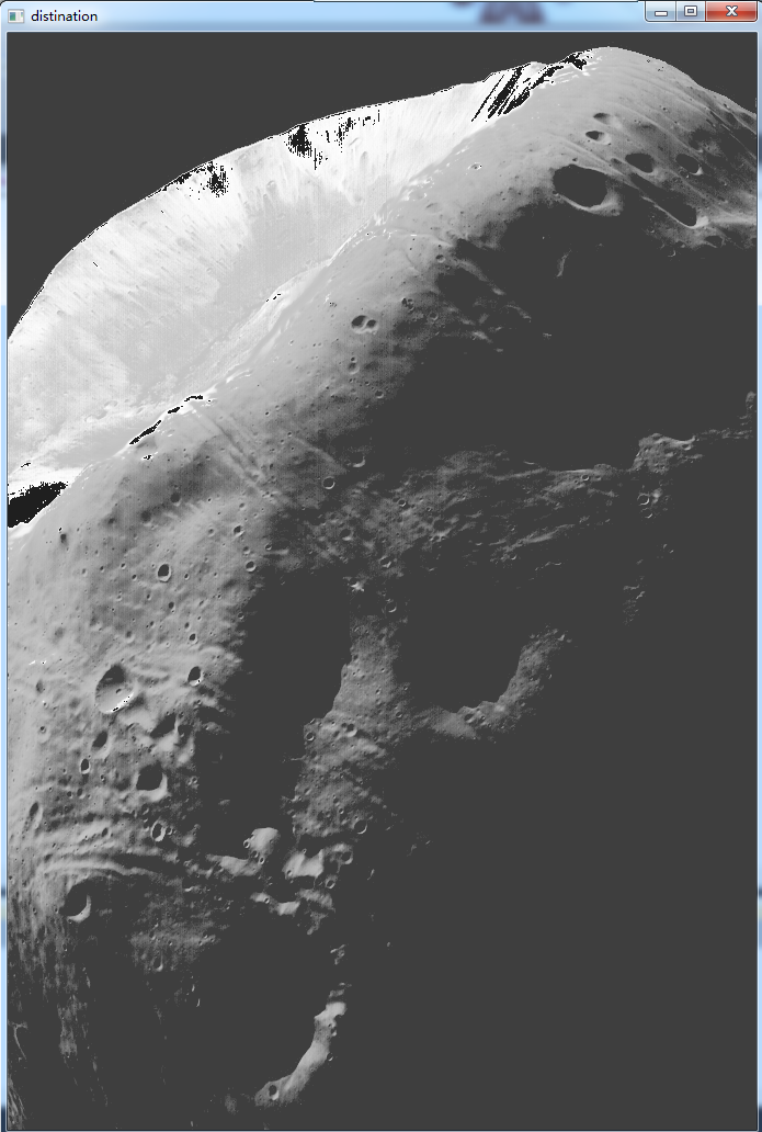 |
图(6)
c++匹配后的效果在某些位置有些失真,也许代码有待调整。
改正代码:
 1 #include "CImg.h"
 2 #include <iostream>
 3 #define K1 0.002
 4 #define A1 1
 5 #define A2 0.07
 6 #define U1 0.15
 7 #define SIG1 0.05
 8 #define U2 0.75
 9 #define SIG2 0.05
10 #define pi 3.1415626535627
11 using namespace cimg_library;
12 /**************直方图匹配*********************************
13 *匹配分布函数:双峰值高斯函数;                            *
14 *图像读取显示库:CImg;                                   *
15 *时间复杂度:O(N^2),操作二维图像,平方级出现在逐像素统计;   *
16 *author:Bruce Mu                                       *
17 *基础测试版                                              *
18 ********************************************************/
19 //双峰值高斯函数
20 inline double twoModeGauss(double r){
21     double w = K1+(A1/sqrt(2*pi)*SIG1)*exp(-(pow((r-U1),2.0)/(2*pow(SIG1,2.0))))+(A2/sqrt(2*pi)*SIG2)*exp(-(pow((r-U2),2.0)/(2*pow(SIG2,2.0))));
22     return w;
23 }
24 void main(int argc,char ** argv)
25 {
26     CImg<unsigned char> img("D:\MATLAB\image\DIP3E_Original_Images_CH03\Fig0323(a)(mars_moon_phobos).tif");
27     int width = img.width();
28     int height = img.height();
29     int consus[257];
30     for(size_t m = 0;m<257;m++){
31         consus[m] = 0;
32     }
33     unsigned sub = 0;
34     double sum = width * height;
35     //统计直方图
36     for(int i = 0;i<width;i++){
37         for(int j = 0;j<height;j++){
38             sub = img(i,j);
39             consus[sub+1]++;
40         }
41     }
42
43     //频数转频率 并求CDF
44     double s[257];
45     s[0] = consus[0]/sum;
46     for(size_t n = 1;n<257;n++){
47         s[n] = s[n-1]+(consus[n]/sum);
48     }
49     //求取指定直方图的CDF
50     double count[257];
51     count[0] = 0;
52     sum = 0;
53     for(size_t a = 0;a<257;a++){
54         double r = (double)a/256.0;
55         count[a+1] = twoModeGauss(r);
56         sum+=count[a+1];
57     }
58     for(size_t c = 1;c<257;c++){
59         count[c]=count[c]/sum;
60     }
61     //根据两个CDF求取灰度映射
62     double v = count[0];
63     unsigned char z[256];
64     size_t p = 1;
65     for(size_t b = 0;b<256;b++){
66         while(s[b]>v){
67             v+=count[p];
68             p++;
69         }
70         z[b] = p;
71     }
72     //按像素点的映射值赋值目标图
73     CImg<unsigned char>dist(img);
74     for(int i = 0;i<width;i++){
75         for(int j = 0;j<height;j++){
76             dist(i,j) = z[img(i,j)];
77         }
78     }
79     //显示
80     CImgDisplay disp1(img,"origin");
81     CImgDisplay disp2(dist,"distination");
82     disp1.wait();
83     disp2.wait();
84 }
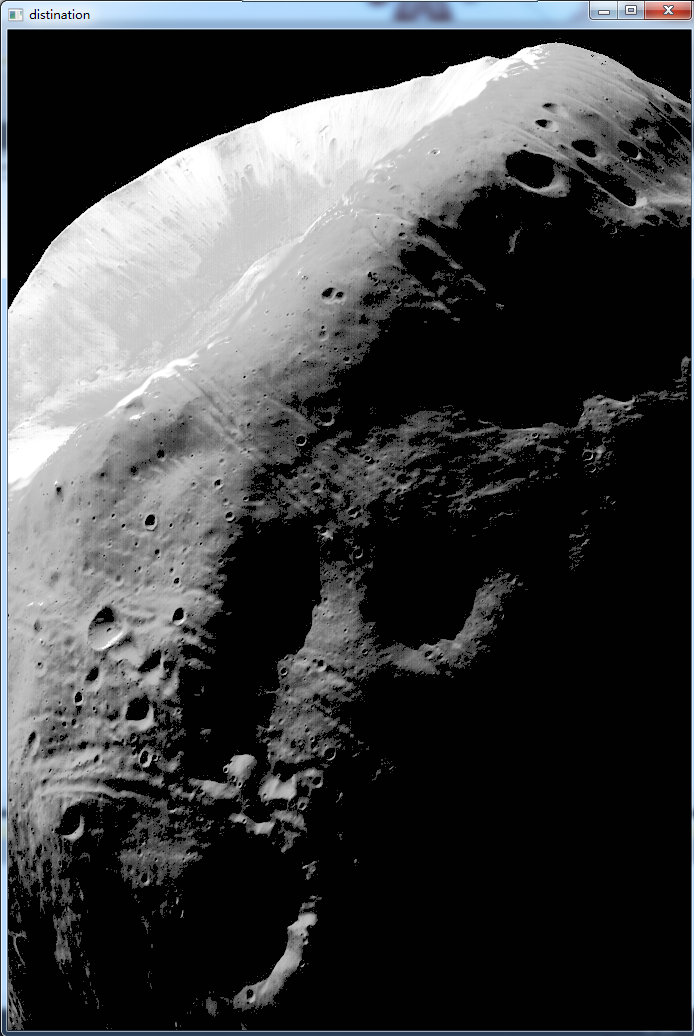
图(7)
局部直方图:
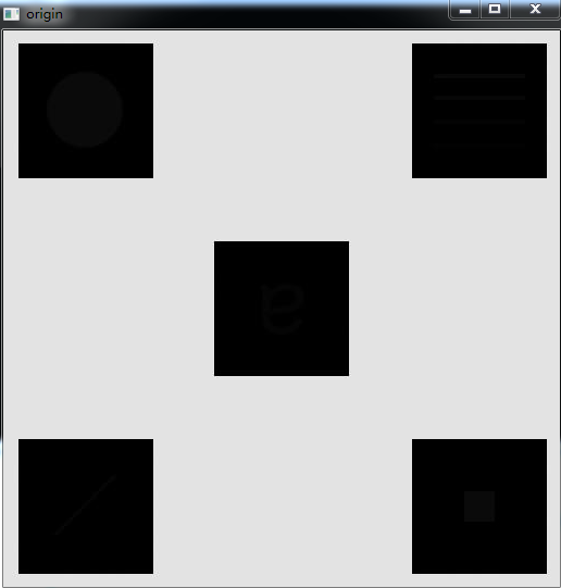
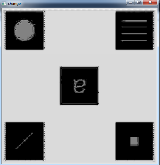
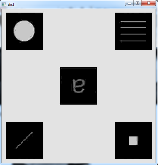
直方图均衡化和直方图匹配都是全局的增强方法,如果对于一些例子,图像的某些部分无需改动,而也存在部分需要增强效果,就需要用到局部直方图。局部直方图的思想在于并非对整个图像采用直方图算法,而是改变目标为针对像素点的邻域。邻域内直方图均衡化或直方图匹配,目的是增强小区域中的细节。这些小区域往往有这样的特点,区域内像素数对全局算法和变换只起到微不足道的作用,所以全局算法很难作用到这样的小区域,而反之小区域内的增强变换并不会影响全局。
实现:逐像素取邻域,应用直方图算法修改中心点像素值;
使用CImg的C局部直方图算法实现:
 1 #include <iostream>
 2 #include "CImg.h"
 3 #include <math.h>
 4 using namespace cimg_library;
 5 //根据统计好的直方图求邻域内的CDF
 6 void getCDF(float *s,const float *const c){
 7     for(size_t i = 1;i<256;i++){
 8         s[i] = s[i-1]+c[i];
 9     }
10 }
11 //局部变换和邻域中心移动后修改统计信息;
12 inline void refresh(float *c,unsigned char sub,BOOL flag){
13     if(flag){
14         c[sub]+=1.0/49.0;
15     }else{
16         c[sub]-=1.0/49.0;
17     }
18 }
19 //应用局部直方图算法
20 void localhist(CImg<unsigned char> &img){
21     int width = img.width();
22     int height = img.height();
23     float count[256];
24     for(size_t t= 0;t<256;t++){
25         count[t]= 0;
26     }
27     //统计第一邻域
28     unsigned char sub = 0;
29     for(int m = 0;m<7;m++){
30         for(int n = 0;n<7;n++){
31             sub = img(m,n);
32             count[sub]+=(1.0/49.0);
33         }
34     }
35     float s[257];
36     s[0] = count[0];
37     getCDF(s,count);
38     sub = img(3,3);
39     unsigned char newvalue = (unsigned char)((s[sub])*255+0.5);
40     img(3,3) = newvalue;
41     refresh(count,sub,false);
42     refresh(count,newvalue,true);
43     //邻域位移,逐邻域修改直方图信息:
44     for(int i = 3;i<height - 4;i++){
45         for(int j = 3;j<width-4;j++){
46             BOOL dirty = true;
47             if(i == 3 && j == 3){
48                 continue;
49             }
50             for(int p = 0;p<7;p++){
51                 unsigned char old =img(j-4,i-3+p);
52                 unsigned char add = img(j+3,i-3+p);
53                 if(old != add){
54                     refresh(count,old,false);
55                     refresh(count,add,true);
56                     dirty = false;
57                 }
58             }
59             if(!dirty){
60                 getCDF(s,count);
61                 sub = img(j,i);
62                 refresh(count,sub,false);
63                 img(j,i) = (unsigned char)(s[sub]*255+0.5);
64                 refresh(count,img(j,i),true);
65             }
66         }
67     }
68 }
69
70 void main(int argc,char **argv){
71     CImg<unsigned char>img("E:\convert.jpeg");
72     CImg<unsigned char>origin(img);
73     CImgDisplay disp1(origin,"origin");
74     localhist(img);
75     CImgDisplay disp2(img,"change");
76     while (!disp1.is_closed() && !disp2.is_closed()) {
77         disp1.wait();
78         disp2.wait();
79     }
80 }
算法效果:
 |
 |
邻域内直方图统计算法:
  1 #include <iostream>
  2 #include "CImg.h"
  3 using namespace std;
  4 using namespace cimg_library;
  5
  6 float getMean(const float *c){
  7     float m = 0;
  8     for(size_t x = 0;x<256;x++){
  9         m+=x*c[x];
 10     }
 11     return m;
 12 }
 13
 14 float getVariance(const float *c,float mean){
 15     float delta = 0;
 16     for(size_t y = 0;y<256;y++){
 17         if(c[y] != 0){
 18             delta += (pow((y-mean),2)*c[y]);
 19         }
 20     }
 21     delta = sqrt(delta);
 22     return delta;
 23 }
 24
 25 void getCount(float *c,int originx,int originy,int wid,int hei,CImg<unsigned char> &img){
 26     for(size_t t = 0;t<256;t++){
 27         c[t] = 0;
 28     }
 29     for(int i = originx;i<wid;i++){
 30         for(int j = originy;j<hei;j++){
 31             unsigned char sub = img(i,j);
 32             c[sub] += 1.0/256.0;
 33         }
 34     }
 35 }
 36
 37 void init(float * count){
 38     for(size_t t = 0;t<256;t++){
 39         count[t] = 0;
 40     }
 41 }
 42 int histStatistic(CImg<unsigned char> &img,int dim,float k0,float k1,float k2,float E){
 43     if(dim%2 == 0){
 44         cout<<"please input a odd num!!!"<<endl;
 45         return -1;
 46     }
 47     int width = img.width();
 48     int height = img.height();
 49     int sum = width * height;
 50     float count[256];
 51     for(size_t t = 0;t<256;t++){
 52         count[t]=0;
 53     }
 54     unsigned char sub = 0;
 55     for(int i = 0;i<width;i++){
 56         for(int j = 0;j<height;j++){
 57             sub = img(i,j);
 58             count[sub]+=1.0/sum;
 59         }
 60     }
 61     float mean = getMean(count);
 62     float delta = getVariance(count,mean);
 63     float mxy = 0;
 64     float deltaxy = 0;
 65     float local = dim*dim;
 66     for(int i = dim/2;i<height - dim/2 -1;i++){
 67         for(int j = dim/2;j<width - dim/2 -1;j++){
 68             //重新初始化统计数组
 69             init(count);
 70             //统计局部直方图
 71             //getCount(count,j-dim/2,i-dim/2,j+dim/2+1,i+dim/2+1,img);
 72             for(int p = j-dim/2;p<j+dim/2+1;p++){
 73                 for(int q = i - dim/2;q < i+dim/2+1;q++){
 74                     sub = img(p,q);
 75                     count[sub] += 1.0/local;
 76                 }
 77             }
 78             mxy = getMean(count);
 79             deltaxy = getVariance(count,mxy);
 80         //    cout<<mxy<<"  :  "<<deltaxy<<endl;
 81             //增强判断
 82             if(mxy <= mean*k0 && deltaxy <=k2*delta && deltaxy >= k1*delta){
 83                 img(j,i) = img(j,i)*E;
 84             //    cout<<"enforcement_________________"<<endl;
 85             }
 86         }
 87     }
 88     return 0;
 89 }
 90
 91 int main(int argc,char ** argv){
 92     CImg<unsigned char> img("E:\statistic.jpeg");
 93     CImg<unsigned char> dist(img);
 94     histStatistic(dist,3,0.4,0.008,0.2,5.0);
 95     CImgDisplay disp1(img,"origin");
 96     CImgDisplay disp2(dist,"dist");
 97     while(!disp1.is_closed() && !disp2.is_closed()){
 98         disp2.wait();
 99     }
100 }
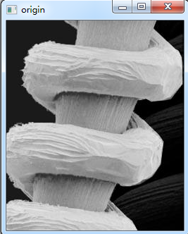
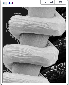
显示效果:
 |
 |
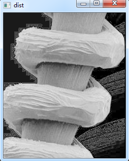 |
调节参数后效果出中仍有白色高亮点,类似椒盐噪声,究其原因是由于本地原图操作造成,如果统计后在另一幅目标图上做修改,效果会比较好,以下是异地操作效果:
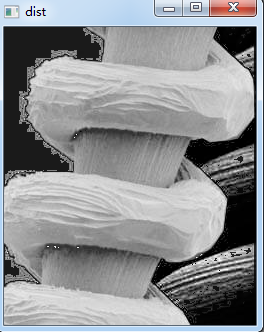
最后,用邻域内直方图统计算法对局部直方图算法中的图像做变换,在参数设置为 邻域为7*7,k0=0.4,k1=0,k2 = 0.4,E =20时的增强效果要好于使用局部直方图,以下是两图的比较:
 |
 |