滤波原理
简而言之,图像的同态滤波是基于以入射光和反射光为基础的图像模型上的,如果把图像函数F(x,y)表示为光照函数,即照射分量i(x,y)与反射分量r(x,y)两个分量的乘积,那么图像的模型可以表示为F(x,y)= i(x,y)*r(x,y)。通过对照射分量i(x,y)和反射分量r(x,y)的研究可知,照射分量一般反映灰度的恒定分量,相当于频域中的低频信息,减弱入射光就可以起到缩小图像灰度范围的作用;而反射光与物体的边界特性是密切相关的,相当于频域中的高频信息,增强反射光就可以起到提高图像对比度的作用。同态滤波器属于频域滤波器范畴,过滤低频信息,放大高频信息,达到压缩图像的灰度空间,并扩展对比度的目的,其传递函数表现为在低频部分小于1,高频部分大于1。具体细节参考Homomorphic filtering
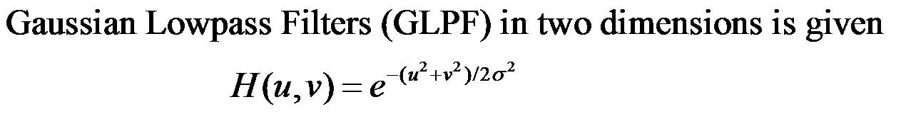
传递函数:H(u,v)

原理流程图:

滤波器设计
根据上述滤波器的特性与传递函数,不难选择滤波器。表达式如图所示。

这里参数c控制上升速率,参考值2,D0参数我们通过高斯低通滤波器来说明,表示的就是横轴截止时的值,如图所示。
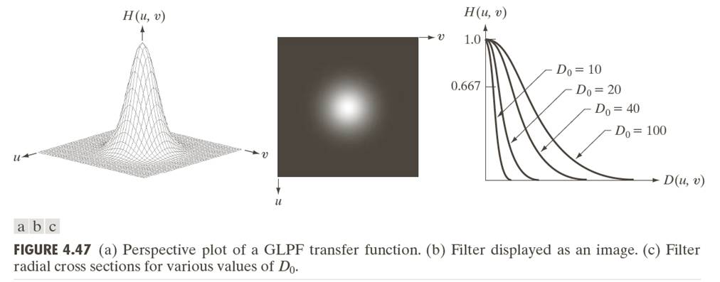
参数D0的选择,是比较讲究的。对应高通滤波器,其决定过滤图像能量的大小。如何自适应取值,我们后面讨论。
OpenCV实现
数据处理
按照上述的原理流程图,第一步需要对数据作相应的处理,然后进行ln取对数操作,这里往往容易出问题。OpenCV读取的图像数据f(x,y)正常是0-255范围的,直接f(x,y)/255.0 + 1.0,然后取对数即可。此处,如果使用normalize函数,然后再加1,后面会发现最终结果g(x,y)是一片黑,原因是normalize对原图的操作是a*f(x,y) + b, 根据傅里叶变换的性质就会发现问题出现在哪里了。DFT
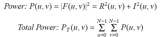
OpenCV中有实现dft的算法,并且在Sample/c++中给出了示例,注意其中将频谱中心移到图像中心的操作。这里补充一点是计算图像的功率谱,还记得上述中提及的D0计算么? 功率谱计算公式如下:
巴特沃斯滤波器
根据求解的参数以及滤波器的传递函数,即可求解出滤波器,此时与DFT的结果一致,滤波器也包含实数与虚数两部分- 频域滤波
调用mulSpectrums进行计算,得到滤波结果,此时注意将结果的频域中心移回到图像的左上角。 - IDFT
OpenCV中有实现idft的算法,注意设置参数DFT_SCALE,具体查看OpenCV的官方文档说明,接着对结果计算e指数,再分解结果的实部和虚部,计算幅值,最后幅值减1. 数据恢复
使用normalize方法,将最大值置为255,并将数据格式转换为CV_8U,得到最终结果。
代码
滤波器:
//High-Frequency-Emphasis Filters
Mat Butterworth_Homomorphic_Filter(Size sz, int D, int n, float high_h_v_TB, float low_h_v_TB,Mat& realIm)
{
    Mat single(sz.height, sz.width, CV_32F);
    cout <<sz.width <<" "<< sz.height<<endl;
    Point centre = Point(sz.height/2, sz.width/2);
    double radius;
    float upper = (high_h_v_TB * 0.1);
    float lower = (low_h_v_TB * 0.1);
    long dpow = D*D;
    float W = (upper - lower);

    for(int i = 0; i < sz.height; i++)
    {
        for(int j = 0; j < sz.width; j++)
        {
            radius = pow((float)(i - centre.x), 2) + pow((float) (j - centre.y), 2);
            float r = exp(-n*radius/dpow);
            if(radius < 0)
                single.at<float>(i,j) = upper;
            else
                single.at<float>(i,j) =W*(1 - r) + lower;
        }
    }

    single.copyTo(realIm);
    Mat butterworth_complex;
    //make two channels to match complex
    Mat butterworth_channels[] = {Mat_<float>(single), Mat::zeros(sz, CV_32F)};
    merge(butterworth_channels, 2, butterworth_complex);

    return butterworth_complex;
}
DFT变换:
//DFT 返回功率谱Power
Mat Fourier_Transform(Mat frame_bw, Mat& image_complex,Mat &image_phase, Mat &image_mag)
{
    Mat frame_log;
    frame_bw.convertTo(frame_log, CV_32F);
    frame_log = frame_log/255;
    /*Take the natural log of the input (compute log(1 + Mag)*/
    frame_log += 1;
    log( frame_log, frame_log); // log(1 + Mag)

    /*2. Expand the image to an optimal size
    The performance of the DFT depends of the image size. It tends to be the fastest for image sizes that are multiple of 2, 3 or 5.
    We can use the copyMakeBorder() function to expand the borders of an image.*/
    Mat padded;
    int M = getOptimalDFTSize(frame_log.rows);
    int N = getOptimalDFTSize(frame_log.cols);
    copyMakeBorder(frame_log, padded, 0, M - frame_log.rows, 0, N - frame_log.cols, BORDER_CONSTANT, Scalar::all(0));

    /*Make place for both the complex and real values
    The result of the DFT is a complex. Then the result is 2 images (Imaginary + Real), and the frequency domains range is much larger than the spatial one. Therefore we need to store in float !
    That's why we will convert our input image "padded" to float and expand it to another channel to hold the complex values.
    Planes is an arrow of 2 matrix (planes[0] = Real part, planes[1] = Imaginary part)*/
    Mat image_planes[] = {Mat_<float>(padded), Mat::zeros(padded.size(), CV_32F)};
    /*Creates one multichannel array out of several single-channel ones.*/
    merge(image_planes, 2, image_complex);

    /*Make the DFT
    The result of thee DFT is a complex image : "image_complex"*/
    dft(image_complex, image_complex);

    /***************************/
    //Create spectrum magnitude//
    /***************************/
    /*Transform the real and complex values to magnitude
    NB: We separe Real part to Imaginary part*/
    split(image_complex, image_planes);
    //Starting with this part we have the real part of the image in planes[0] and the imaginary in planes[1]
    phase(image_planes[0], image_planes[1], image_phase);
    magnitude(image_planes[0], image_planes[1], image_mag);

    //Power
    pow(image_planes[0],2,image_planes[0]);
    pow(image_planes[1],2,image_planes[1]);

    Mat Power = image_planes[0] + image_planes[1];

    return Power;
}
IDFT变换
void Inv_Fourier_Transform(Mat input, Mat& inverseTransform)
{
    /*Make the IDFT*/
    Mat result;
    idft(input, result,DFT_SCALE);
    /*Take the exponential*/
    exp(result, result);

    vector<Mat> planes;
    split(result,planes);
    magnitude(planes[0],planes[1],planes[0]);
    planes[0] = planes[0] - 1.0;
    normalize(planes[0],planes[0],0,255,CV_MINMAX);

    planes[0].convertTo(inverseTransform,CV_8U);
}
频谱移位
//SHIFT
void Shifting_DFT(Mat &fImage)
{
    //For visualization purposes we may also rearrange the quadrants of the result, so that the origin (0,0), corresponds to the image center.
    Mat tmp, q0, q1, q2, q3;

    /*First crop the image, if it has an odd number of rows or columns.
    Operator & bit to bit by -2 (two's complement : -2 = 111111111....10) to eliminate the first bit 2^0 (In case of odd number on row or col, we take the even number in below)*/
    fImage = fImage(Rect(0, 0, fImage.cols & -2, fImage.rows & -2));
    int cx = fImage.cols/2;
    int cy = fImage.rows/2;

    /*Rearrange the quadrants of Fourier image so that the origin is at the image center*/
    q0 = fImage(Rect(0, 0, cx, cy));
    q1 = fImage(Rect(cx, 0, cx, cy));
    q2 = fImage(Rect(0, cy, cx, cy));
    q3 = fImage(Rect(cx, cy, cx, cy));

    /*We reverse each quadrant of the frame with its other quadrant diagonally opposite*/
    /*We reverse q0 and q3*/
    q0.copyTo(tmp);
    q3.copyTo(q0);
    tmp.copyTo(q3);

    /*We reverse q1 and q2*/
    q1.copyTo(tmp);
    q2.copyTo(q1);
    tmp.copyTo(q2);
}
主函数:
void homomorphicFiltering(Mat src,Mat& dst)
{
    Mat img;
    Mat imgHls;
    vector<Mat> vHls;

    if(src.channels() == 3)
    {
        cvtColor(src,imgHls,CV_BGR2HSV);
        split(imgHls,vHls);
        vHls[2].copyTo(img);
    }
    else
        src.copyTo(img);

    //DFT
    //cout<<"DFT "<<endl;
    Mat img_complex,img_mag,img_phase;
    Mat fpower = Fourier_Transform(img,img_complex,img_phase,img_mag);
    Shifting_DFT(img_complex);
    Shifting_DFT(fpower);
    //int D0 = getRadius(fpower,0.15);
    int D0 = 10;
    int n = 2;
    int w = img_complex.cols;
    int h = img_complex.rows;
    //BHPF
//  Mat filter,filter_complex;
//  filter = BHPF(h,w,D0,n);
//  Mat planes[] = {Mat_<float>(filter), Mat::zeros(filter.size(), CV_32F)};
//  merge(planes,2,filter_complex);

    int rH = 150;
    int rL = 50;
    Mat filter,filter_complex;
    filter_complex = Butterworth_Homomorphic_Filter(Size(w,h),D0,n,rH,rL,filter);

    //do mulSpectrums on the full dft
    mulSpectrums(img_complex, filter_complex, filter_complex, 0);

    Shifting_DFT(filter_complex);
    //IDFT
    Mat result;
    Inv_Fourier_Transform(filter_complex,result);

    if(src.channels() == 3)
    {
        vHls.at(2)= result(Rect(0,0,src.cols,src.rows));
        merge(vHls,imgHls);
        cvtColor(imgHls, dst, CV_HSV2BGR);
    }
    else
        result.copyTo(dst);

}