基础矩阵-Python

基础矩阵

　　基础矩阵 F 可以由两照相机的参数矩阵（相对旋转 R 和平移 t）表示，我们可以借助 F 来恢复出照相机参数，而 F 可以从对应的投影图像点计算出来，它体现了两视图几何（对极几何）的内在射影几何关系即基础矩阵描述了空间中的点在两个像平面中的坐标对应关系。

对极几何

在上一篇相机模型里我们知道x=PX。通过小孔相机模型，可知从相机的中心C向点x投影一条射线Cx，则该射线必定经过对应像点的三维空间点X，但显然仅仅通过一个像点无法确定X的具体位置。那么如果两个相匹配的像点呢？
设x′是三维点X的另一个像点，其对应相机的中心为C′，那么从相机的中心C′向点也投影一条射线C′x′，并且该射线也必定经过X，也就是说从一对相匹配的像点反投影两条射线，必定相交于空间三维点X。那么一对匹配的像点之间存在这某种约束关系，这种约束被称为两视图的对极约束。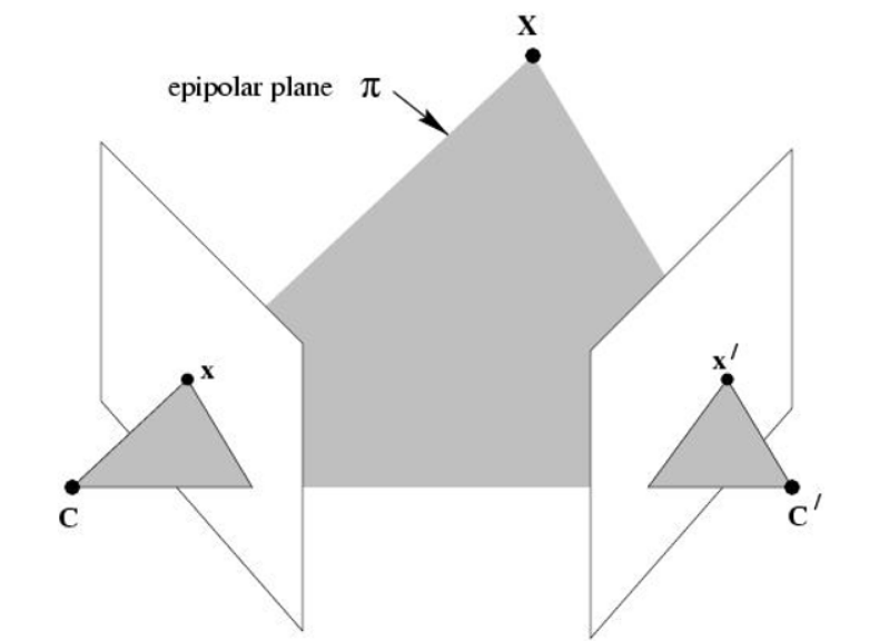

8点算法

8点算法是计算基本矩阵（两幅图像之间的约束关系使用代数的方式表示出来即为基本矩阵）的最简单的方法，它仅涉及构造并（最小二乘）解一个线性方程组，如果小心的话，它可以执行得非常好。8点算法成功的关键是在构造解的方程之前应对输入的数据认真进行适当的归一化。在形成8点算法的线性方程组之前，图像点的一个简单变换（平移或变尺度）将使这个问题的条件极大的改善，从而提高结果的稳定性，而且进行这种变换所增加的计算复杂性并不显著。

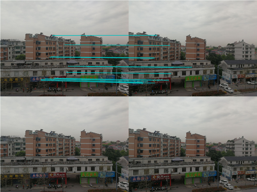
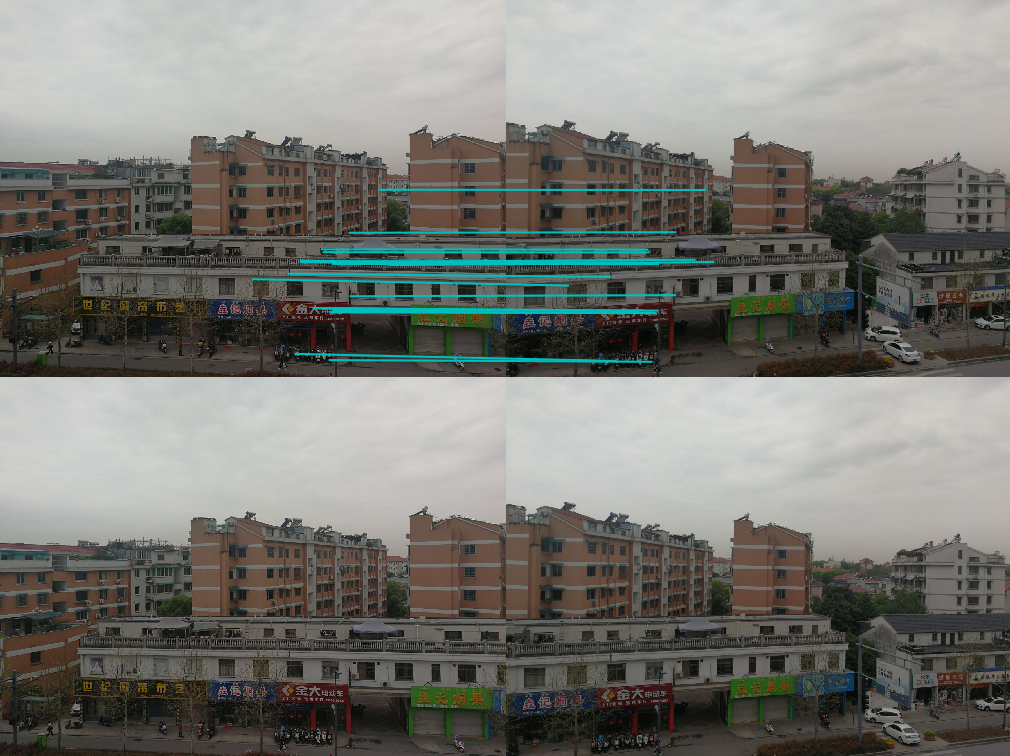
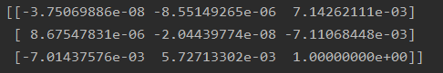
像平面接近平行，极点位于无穷远

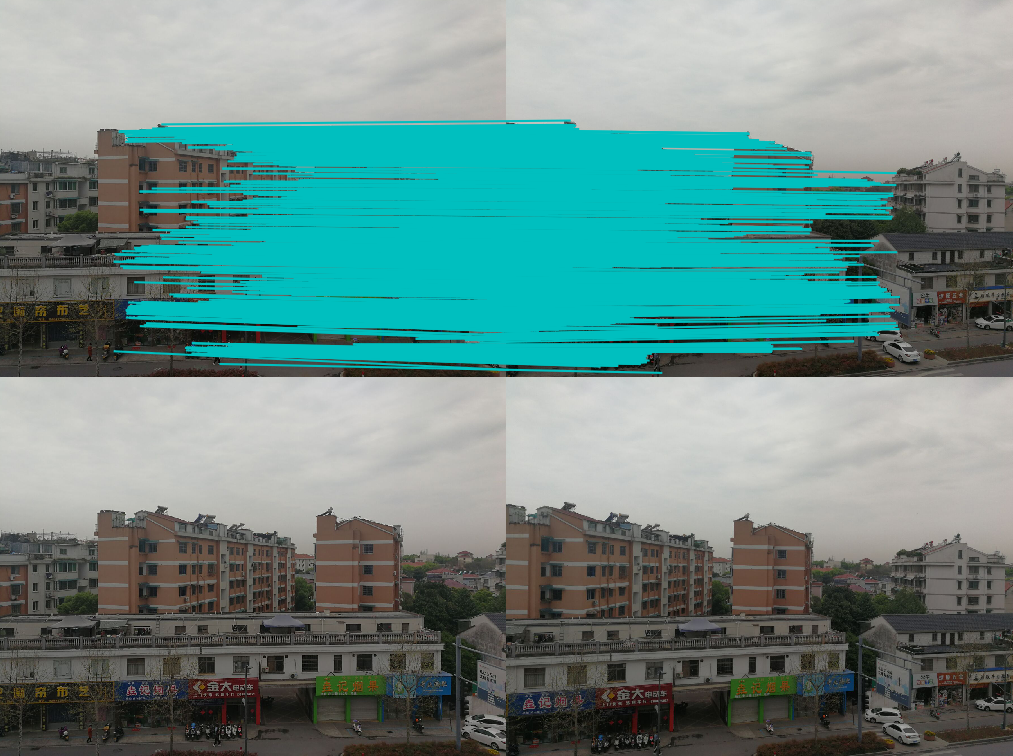
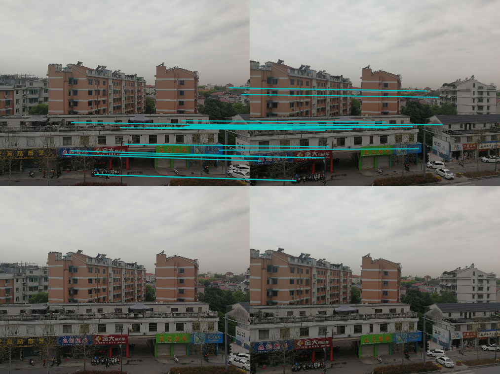
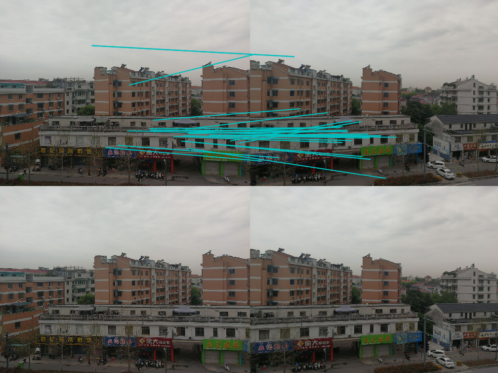
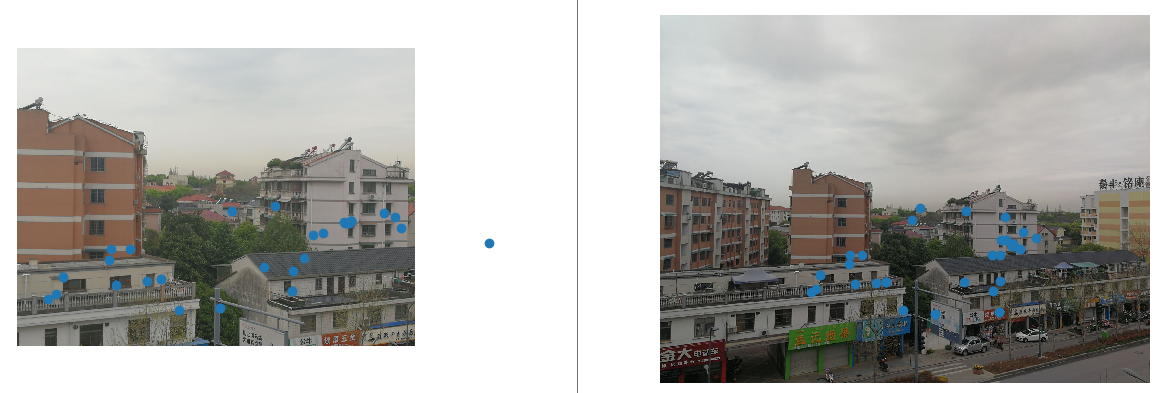
sift特征点匹配效果

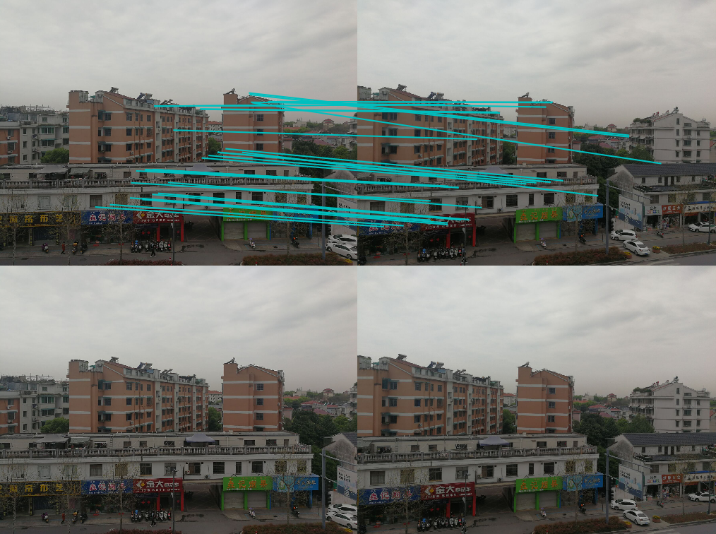
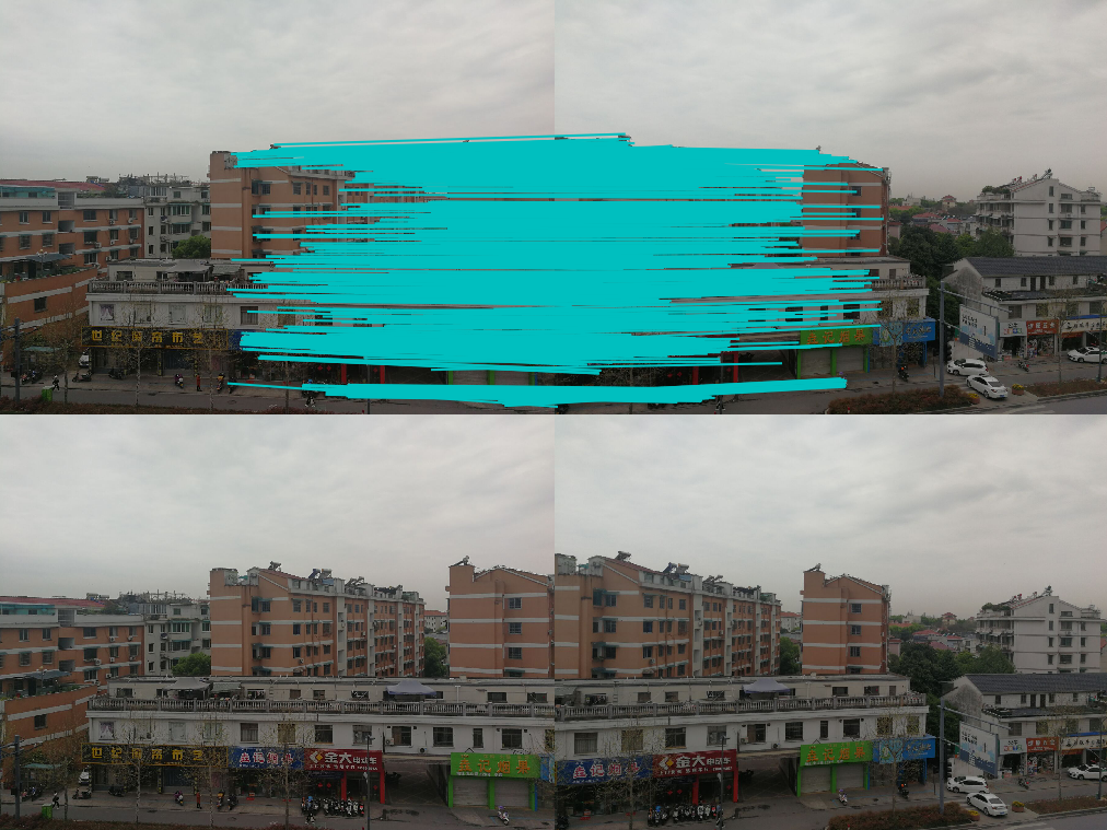
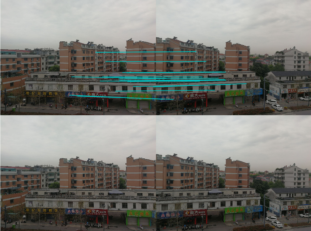
ransac算法优化

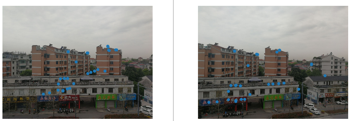
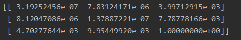
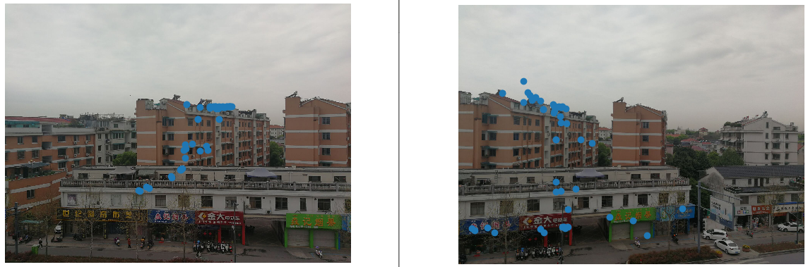
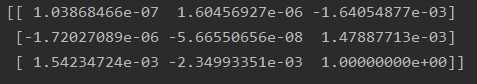
8点算法结果

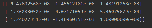
基础矩阵：

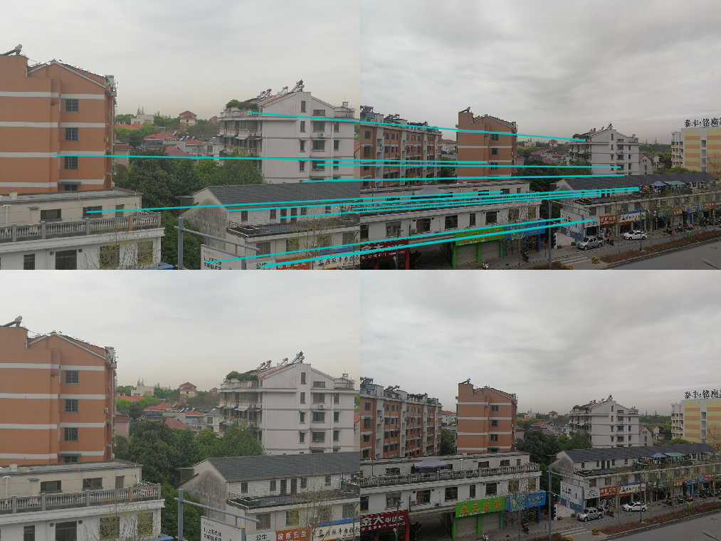
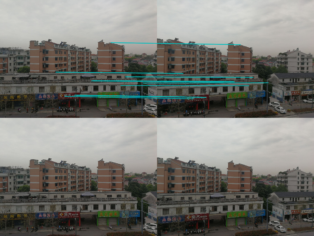
左右拍摄，极点位于图像平面上

sift特征点匹配效果

ransac算法优化

8点算法结果

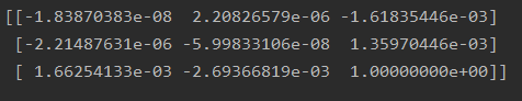
基础矩阵：

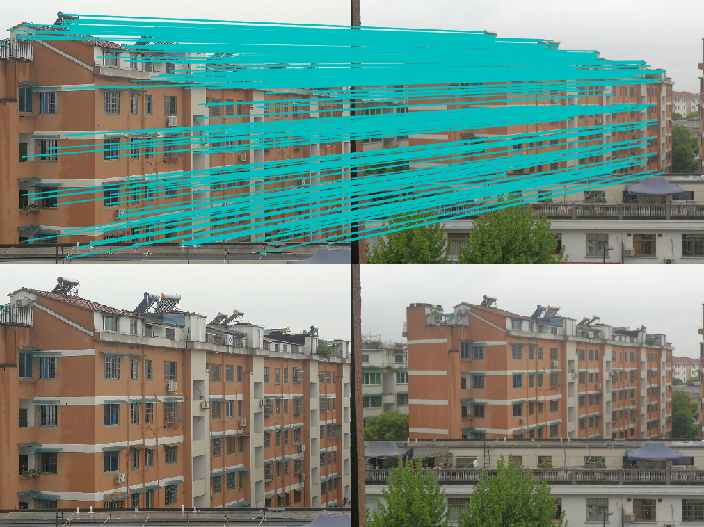
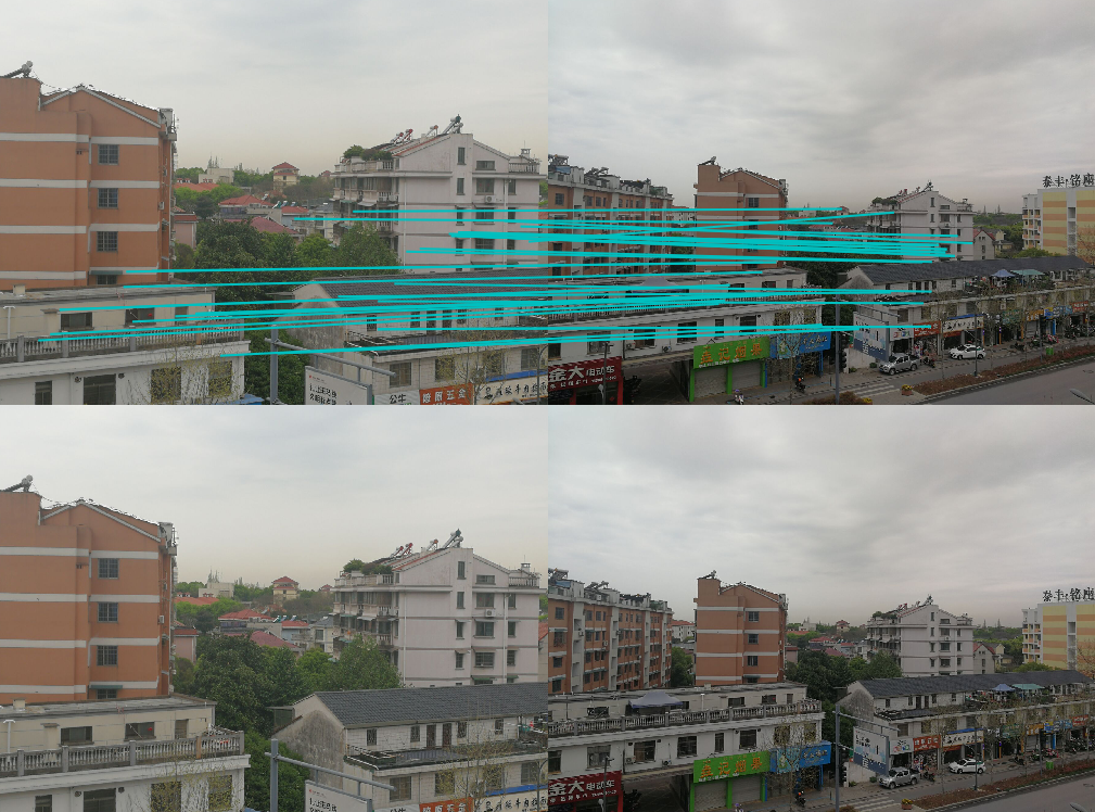
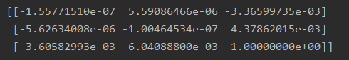
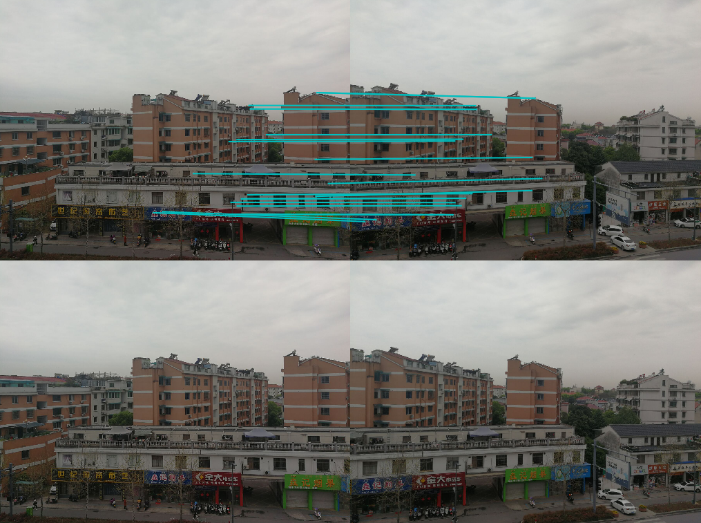
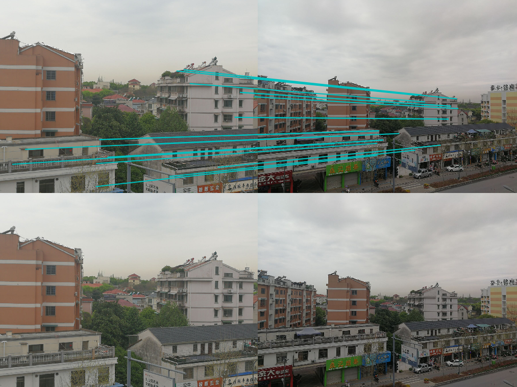
图像拍摄位置位于前后

sift特征点匹配效果

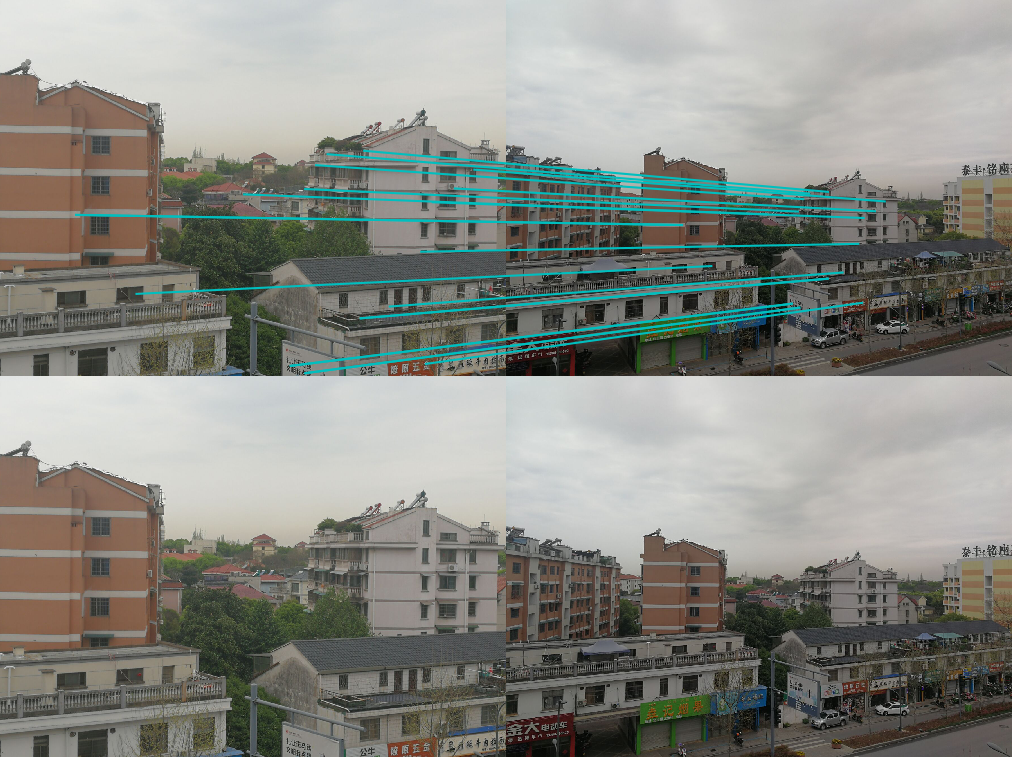
ransac算法优化

8点算法结果

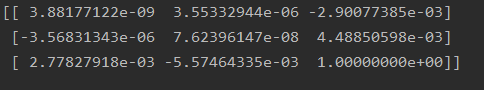
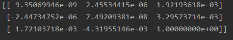
基础矩阵：

七点算法

像平面接近平行，极点位于无穷远

左右拍摄，极点位于图像平面上

图像拍摄位置位于前后

十点算法

像平面接近平行，极点位于无穷远

左右拍摄，极点位于图像平面上

图像拍摄位置位于前后

总结

照片的拍摄距离有些远，匹配的效果不是很好，有错误的匹配点较多，试着缩小拍摄距离会降低错误的匹配点，也可以提升图片的质量， 2-3M的图片匹配起来最好，但是相应的程序运行的时间成本就更大，优化后的特征点也更正确。
有时候会因为匹配点附近太过相似而出现错误匹配，即使是经过优化后的结果仍存在错误的匹配点，图像拍摄的远近、明暗、质量都影响最终的结果
8点算法是计算基本矩阵的最简单的方法，稳定性和精度都比7点、10点算法要好，而且运行速度也是较快的，7点算法反而最慢，不知道是不是我图片的质量影响了运行速度
可能是我的图片边缘都不是很工整，较为平滑，导致特征点都没有匹配对，也有可能是背景墙面的花纹特征点更为明显，匹配的时候有限匹配了墙面的特征点。建议拍摄图片时选择墙面没有花纹的好一些。

报错

E:PyCharm 2018.2.5helperspycharmdocrunner.py:1: DeprecationWarning: the imp module is deprecated in favour of importlib; see the module's documentation for alternative uses import imp

这是因为imp 从 Python 3.4 之后弃用了，建议使用 importlib 代替

解决方法一：

打开 Pycharm安装目录pycharmdocrunner.py 文件，做如下两步修改

在第一行，注释掉 imp，导入 importlib

在第 230 行的 loadSource 函数中，注释 imp.load_source，使用 importlib.machinery.SourceFileLoader 加载模块

解决方法二：

在导入包的位置，将imp改成importlib

-->

报错直接解除，不过我不知道对低版本的python有没有用，最好用方法一处理。

出现 ValueError: did not meet fit acceptance criteria 的错误，这是由于拍摄的图像水平落差比较大，可以重新拍摄一组图像。

代码：

# -*- coding: utf-8 -*-
from PIL import Image
from numpy import *
from pylab import *
import numpy as np
from PCV.geometry import camera
from PCV.geometry import homography
from PCV.geometry import sfm
from PCV.localdescriptors import sift
# -*- coding: utf-8 -*-

# Read features
# 载入图像，并计算特征
im1 = array(Image.open('E:/test_pic/jichujuzhen/1.jpg'))
sift.process_image('E:/test_pic/jichujuzhen/1.jpg', 'E:/test_pic/jichujuzhen/im1.sift')
l1, d1 = sift.read_features_from_file('E:/test_pic/jichujuzhen/im1.sift')

im2 = array(Image.open('E:/test_pic/jichujuzhen/2.jpg'))
sift.process_image('E:/test_pic/jichujuzhen/2.jpg', 'E:/test_pic/jichujuzhen/im2.sift')
l2, d2 = sift.read_features_from_file('E:/test_pic/jichujuzhen/im2.sift')

# 匹配特征
matches = sift.match_twosided(d1, d2)
ndx = matches.nonzero()[0]

# 使用齐次坐标表示，并使用 inv(K) 归一化
x1 = homography.make_homog(l1[ndx, :2].T)
ndx2 = [int(matches[i]) for i in ndx]
x2 = homography.make_homog(l2[ndx2, :2].T)

x1n = x1.copy()
x2n = x2.copy()
print(len(ndx))

figure(figsize=(16,16))
sift.plot_matches(im1, im2, l1, l2, matches, True)
show()

# Don't use K1, and K2

#def F_from_ransac(x1, x2, model, maxiter=5000, match_threshold=1e-6):
def F_from_ransac(x1, x2, model, maxiter=5000, match_threshold=1e-6):
    """ Robust estimation of a fundamental matrix F from point
    correspondences using RANSAC (ransac.py from
    http://www.scipy.org/Cookbook/RANSAC).

    input: x1, x2 (3*n arrays) points in hom. coordinates. """

    from PCV.tools import ransac
    data = np.vstack((x1, x2))
    d = 20 # 20 is the original
    # compute F and return with inlier index
    F, ransac_data = ransac.ransac(data.T, model, 8, maxiter, match_threshold, d, return_all=True)
    return F, ransac_data['inliers']

# find E through RANSAC
# 使用 RANSAC 方法估计 E
model = sfm.RansacModel()
F, inliers = F_from_ransac(x1n, x2n, model, maxiter=5000, match_threshold=1e-4)
print(len(x1n[0]))
print(len(inliers))

# 计算照相机矩阵（P2 是 4 个解的列表）
P1 = array([[1, 0, 0, 0], [0, 1, 0, 0], [0, 0, 1, 0]])
P2 = sfm.compute_P_from_fundamental(F)

# triangulate inliers and remove points not in front of both cameras
X = sfm.triangulate(x1n[:, inliers], x2n[:, inliers], P1, P2)

# plot the projection of X
cam1 = camera.Camera(P1)
cam2 = camera.Camera(P2)
x1p = cam1.project(X)
x2p = cam2.project(X)

figure()
imshow(im1)
gray()
plot(x1p[0], x1p[1], 'o')
#plot(x1[0], x1[1], 'r.')
axis('off')

figure()
imshow(im2)
gray()
plot(x2p[0], x2p[1], 'o')
#plot(x2[0], x2[1], 'r.')
axis('off')
show()

figure(figsize=(16, 16))
im3 = sift.appendimages(im1, im2)
im3 = vstack((im3, im3))

imshow(im3)

cols1 = im1.shape[1]
rows1 = im1.shape[0]
for i in range(len(x1p[0])):
    if (0<= x1p[0][i]<cols1) and (0<= x2p[0][i]<cols1) and (0<=x1p[1][i]<rows1) and (0<=x2p[1][i]<rows1):
        plot([x1p[0][i], x2p[0][i]+cols1],[x1p[1][i], x2p[1][i]],'c')
axis('off')
show()

print(F)

x1e = []
x2e = []
ers = []
for i,m in enumerate(matches):
    if m>0: #plot([locs1[i][0],locs2[m][0]+cols1],[locs1[i][1],locs2[m][1]],'c')
        x1=int(l1[i][0])
        y1=int(l1[i][1])
        x2=int(l2[int(m)][0])
        y2=int(l2[int(m)][1])
        # p1 = array([l1[i][0], l1[i][1], 1])
        # p2 = array([l2[m][0], l2[m][1], 1])
        p1 = array([x1, y1, 1])
        p2 = array([x2, y2, 1])
        # Use Sampson distance as error
        Fx1 = dot(F, p1)
        Fx2 = dot(F, p2)
        denom = Fx1[0]**2 + Fx1[1]**2 + Fx2[0]**2 + Fx2[1]**2
        e = (dot(p1.T, dot(F, p2)))**2 / denom
        x1e.append([p1[0], p1[1]])
        x2e.append([p2[0], p2[1]])
        ers.append(e)
x1e = array(x1e)
x2e = array(x2e)
ers = array(ers)

indices = np.argsort(ers)
x1s = x1e[indices]
x2s = x2e[indices]
ers = ers[indices]
x1s = x1s[:20]
x2s = x2s[:20]

figure(figsize=(16, 16))
im3 = sift.appendimages(im1, im2)
im3 = vstack((im3, im3))

imshow(im3)

cols1 = im1.shape[1]
rows1 = im1.shape[0]
for i in range(len(x1s)):
    if (0<= x1s[i][0]<cols1) and (0<= x2s[i][0]<cols1) and (0<=x1s[i][1]<rows1) and (0<=x2s[i][1]<rows1):
        plot([x1s[i][0], x2s[i][0]+cols1],[x1s[i][1], x2s[i][1]],'c')
axis('off')
show()