SVM介绍
def L(x,y,w):
    scores = W.dot(x)
    margins = np.maximum(0,scores - scores[y] + 1)
    margins[y] = 0
    loss_i = np.sum(margins)
    return loss_i
linear_svm.py
import numpy as np
from random import shuffle

def svm_loss_naive(W, X, y, reg):
  """
  Structured SVM loss function, naive implementation (with loops).

  Inputs have dimension D, there are C classes, and we operate on minibatches
  of N examples.

  Inputs:
  - W: A numpy array of shape (D, C) containing weights.
  - X: A numpy array of shape (N, D) containing a minibatch of data.
  - y: A numpy array of shape (N,) containing training labels; y[i] = c means
    that X[i] has label c, where 0 <= c < C.
  - reg: (float) regularization strength 正则化强度

  Returns a tuple of:
  - loss as single float
  - gradient with respect to weights W; an array of same shape as W
  """
  dW = np.zeros(W.shape) # initialize the gradient as zero
  # dw (3073,10) 3073=3072+1 因为预处理(添加一列1作为偏置维度,这样我们在优化时候只要考虑一个权重矩阵W就可以啦.)
  # compute the loss and the gradient
  num_classes = W.shape[1] #10
  num_train = X.shape[0] #X (500,3073)
  loss = 0.0
  for i in range(num_train):
    scores = X[i].dot(W)
    # scores (10,1) 代表对于每一类的分数
    correct_class_score = scores[y[i]]
    #y[i]=c 表示 x[i]的标签为c,其中 0 <= c <= C,correct_class_score即正确标签那一类的分数
    for j in range(num_classes):
      if j == y[i]: #跳过同类的那一个
        continue
      margin = scores[j] - correct_class_score + 1 # note delta = 1
      if margin > 0:
        loss += margin
        dW[:, y[i]] += -X[i, :]     #  根据公式:∇Wyi Li = - xiT(∑j≠yi1(xiWj - xiWyi +1>0)) + 2λWyi
        dW[:, j] += X[i, :]         #  根据公式: ∇Wj Li = xiT 1(xiWj - xiWyi +1>0) + 2λWj , (j≠yi)
  # Right now the loss is a sum over all training examples, but we want it
  # to be an average instead so we divide by num_train.
  loss /= num_train
  dW /= num_train

  # Add regularization to the loss.
  loss += reg * np.sum(W * W)
  dW += reg * W
  #############################################################################
  # TODO:                                                                     #
  # Compute the gradient of the loss function and store it dW.                #
  # Rather that first computing the loss and then computing the derivative,   #
  # it may be simpler to compute the derivative at the same time that the     #
  # loss is being computed. As a result you may need to modify some of the    #
  # code above to compute the gradient.                                       #
  #############################################################################


  return loss, dW


def svm_loss_vectorized(W, X, y, reg):
  """
  Structured SVM loss function, vectorized implementation.

  Inputs and outputs are the same as svm_loss_naive.
  """
  loss = 0.0
  dW = np.zeros(W.shape) # initialize the gradient as zero

  #############################################################################
  # TODO:                                                                     #
  # Implement a vectorized version of the structured SVM loss, storing the    #
  # result in loss.                                                           #
  #############################################################################
  scores = X.dot(W)
  #scores(500,10)即(N,C),存储每个类的分数
  num_classes = W.shape[1]
  num_train = X.shape[0] #num_train = N
  scores_correct = scores[np.arange(num_train),y]
  #scores_correct(1,N) y(N,1) 即对于每个训练样本,找到正确标签那一类的分数 np.arange(num_train)和y分别作为scores的系数
  scores_correct = np.reshape(scores_correct,(num_train,-1))
  #scores_correct(N,1)
  margins = scores - scores_correct + 1
  # scores(N,C) scores_correct(N,1)  减法的方法是scores[i]中每一维都减去scores_correct[i]
  # margins(N,C)
  margins = np.maximum(0,margins)
  #对每个元素取max(0,x)
  margins[np.arange(num_train),y] = 0
  # 跳过同类的那一个
  loss += np.sum(margins) / num_train #要除以训练集个数
  loss += 0.5 * reg * np.sum(W * W) #正则项
  #############################################################################
  #                             END OF YOUR CODE                              #
  #############################################################################


  #############################################################################
  # TODO:                                                                     #
  # Implement a vectorized version of the gradient for the structured SVM     #
  # loss, storing the result in dW.                                           #
  #                                                                           #
  # Hint: Instead of computing the gradient from scratch, it may be easier    #
  # to reuse some of the intermediate values that you used to compute the     #
  # loss.                                                                     #
  #############################################################################
  margins[margins > 0] = 1
  #大于0的采用求导数
  row_sum = np.sum(margins,axis = 1)
  #row_sum(1,N) margins中每一行的和
  margins[np.arange(num_train),y] = -row_sum
  #对于正确标签那一类的梯度计算不同于其它类
  dW += np.dot(X.T,margins)/num_train + reg*W
  #############################################################################
  #                             END OF YOUR CODE                              #
  #############################################################################

  return loss, dW
linear_classifier.py
使用随机梯度下降来训练
from __future__ import print_function

import numpy as np
from cs231n.classifiers.linear_svm import *
from cs231n.classifiers.softmax import *

class LinearClassifier(object):

  def __init__(self):
    self.W = None

  def train(self, X, y, learning_rate=1e-3, reg=1e-5, num_iters=100,
            batch_size=200, verbose=False):
    #verbose 若为真,优化时打印过程。
    """
    Train this linear classifier using stochastic gradient descent.

    Inputs:
    - X: A numpy array of shape (N, D) containing training data; there are N
      training samples each of dimension D.
    - y: A numpy array of shape (N,) containing training labels; y[i] = c
      means that X[i] has label 0 <= c < C for C classes.
    - learning_rate: (float) learning rate for optimization.
    - reg: (float) regularization strength.
    - num_iters: (integer) number of steps to take when optimizing
    - batch_size: (integer) number of training examples to use at each step.
    - verbose: (boolean) If true, print progress during optimization.

    Outputs:
    A list containing the value of the loss function at each training iteration.
    """
    num_train, dim = X.shape
    num_classes = np.max(y) + 1 # assume y takes values 0...K-1 where K is number of classes
    if self.W is None:
      # lazily initialize W
      self.W = 0.001 * np.random.randn(dim, num_classes)

    # Run stochastic gradient descent to optimize W
    loss_history = []
    for it in range(num_iters):
      X_batch = None
      y_batch = None

      #########################################################################
      # TODO:                                                                 #
      # Sample batch_size elements from the training data and their           #
      # corresponding labels to use in this round of gradient descent.        #
      # Store the data in X_batch and their corresponding labels in           #
      # y_batch; after sampling X_batch should have shape (dim, batch_size)   #
      # and y_batch should have shape (batch_size,)                           #
      #                                                                       #
      # Hint: Use np.random.choice to generate indices. Sampling with         #
      # replacement is faster than sampling without replacement.              #
      #########################################################################
      batch_inx = np.random.choice(num_train,batch_size)
      X_batch = X[batch_inx,:]
      y_batch = y[batch_inx]
      #采样
      #########################################################################
      #                       END OF YOUR CODE                                #
      #########################################################################

      # evaluate loss and gradient
      loss, grad = self.loss(X_batch, y_batch, reg)
      loss_history.append(loss)

      # perform parameter update
      #########################################################################
      # TODO:                                                                 #
      # Update the weights using the gradient and the learning rate.          #
      #########################################################################
      self.W = self.W - learning_rate * grad
      #########################################################################
      #                       END OF YOUR CODE                                #
      #########################################################################

      if verbose and it % 100 == 0:
        print('iteration %d / %d: loss %f' % (it, num_iters, loss))

    return loss_history

  def predict(self, X):
    """
    Use the trained weights of this linear classifier to predict labels for
    data points.

    Inputs:
    - X: A numpy array of shape (N, D) containing training data; there are N
      training samples each of dimension D.

    Returns:
    - y_pred: Predicted labels for the data in X. y_pred is a 1-dimensional
      array of length N, and each element is an integer giving the predicted
      class.
    """
    y_pred = np.zeros(X.shape[0])
    ###########################################################################
    # TODO:                                                                   #
    # Implement this method. Store the predicted labels in y_pred.            #
    ###########################################################################
    y_pred = np.argmax(np.dot(X,self.W),axis = 1)
    # X(N,D) W(D,C) y_pred(N,1)
    ###########################################################################
    #                           END OF YOUR CODE                              #
    ###########################################################################
    return y_pred

  def loss(self, X_batch, y_batch, reg):
    """
    Compute the loss function and its derivative.
    Subclasses will override this.

    Inputs:
    - X_batch: A numpy array of shape (N, D) containing a minibatch of N
      data points; each point has dimension D.
    - y_batch: A numpy array of shape (N,) containing labels for the minibatch.
    - reg: (float) regularization strength.

    Returns: A tuple containing:
    - loss as a single float
    - gradient with respect to self.W; an array of the same shape as W
    """
    pass


class LinearSVM(LinearClassifier):
  """ A subclass that uses the Multiclass SVM loss function """

  def loss(self, X_batch, y_batch, reg):
    return svm_loss_vectorized(self.W, X_batch, y_batch, reg)


class Softmax(LinearClassifier):
  """ A subclass that uses the Softmax + Cross-entropy loss function """

  def loss(self, X_batch, y_batch, reg):
    return softmax_loss_vectorized(self.W, X_batch, y_batch, reg)
cross-validation部分:
# Use the validation set to tune hyperparameters (regularization strength and
# learning rate). You should experiment with different ranges for the learning
# rates and regularization strengths; if you are careful you should be able to
# get a classification accuracy of about 0.4 on the validation set.
learning_rates = [1e-7, 5e-5]
regularization_strengths = [2.5e4, 5e4]

# results is dictionary mapping tuples of the form
# (learning_rate, regularization_strength) to tuples of the form
# (training_accuracy, validation_accuracy). The accuracy is simply the fraction
# of data points that are correctly classified.
results = {}
best_val = -1   # The highest validation accuracy that we have seen so far.
best_svm = None # The LinearSVM object that achieved the highest validation rate.

################################################################################
# TODO:                                                                        #
# Write code that chooses the best hyperparameters by tuning on the validation #
# set. For each combination of hyperparameters, train a linear SVM on the      #
# training set, compute its accuracy on the training and validation sets, and  #
# store these numbers in the results dictionary. In addition, store the best   #
# validation accuracy in best_val and the LinearSVM object that achieves this  #
# accuracy in best_svm.                                                        #
#                                                                              #
# Hint: You should use a small value for num_iters as you develop your         #
# validation code so that the SVMs don't take much time to train; once you are #
# confident that your validation code works, you should rerun the validation   #
# code with a larger value for num_iters.                                      #
################################################################################
for rate in learning_rates:
    for regular in regularization_strengths:
        svm = LinearSVM()
        svm.train(X_train,y_train,learning_rate = rate,reg = regular,num_iters = 1000)
        y_train_pred = svm.predict(X_train)
        accuracy_train = np.mean(y_train == y_train_pred)
        y_val_pred = svm.predict(X_val)
        accuracy_val = np.mean(y_val == y_val_pred)
        results[(rate,regular)] = (accuracy_train,accuracy_val)
        if best_val < accuracy_val:
            best_val = accuracy_val
            best_svm = svm
################################################################################
#                              END OF YOUR CODE                                #
################################################################################

# Print out results.
for lr, reg in sorted(results):
    train_accuracy, val_accuracy = results[(lr, reg)]
    print('lr %e reg %e train accuracy: %f val accuracy: %f' % (
                lr, reg, train_accuracy, val_accuracy))

print('best validation accuracy achieved during cross-validation: %f' % best_val)
Note:
-
- dot mul
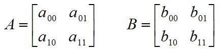
- A*B 矩阵乘法,返回矩阵
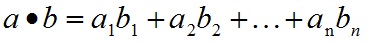
- A.dot(B) 內积,返回一个标量
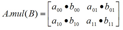
- A.mul(B) 要求A和B的形状一致,对应元素的乘法。
参考:https://blog.csdn.net/dcrmg/article/details/52404580

- np.arrange
返回值: np.arange()函数返回一个有终点和起点的固定步长的排列,如[1,2,3,4,5],起点是1,终点是5,步长为1。
参数个数情况: np.arange()函数分为一个参数,两个参数,三个参数三种情况
1)一个参数时,参数值为终点,起点取默认值0,步长取默认值1。
2)两个参数时,第一个参数为起点,第二个参数为终点,步长取默认值1。
3)三个参数时,第一个参数为起点,第二个参数为终点,第三个参数为步长。其中步长支持小数。
#一个参数 默认起点0,步长为1 输出:[0 1 2]
a = np.arange(3)

#两个参数 默认步长为1 输出[3 4 5 6 7 8]
a = np.arange(3,9)

#三个参数 起点为0,终点为4,步长为0.1 输出[ 0.   0.1  0.2  0.3  0.4  0.5  0.6  0.7  0.8  0.9  1.   1.1  1.2  1.3  1.4 1.5  1.6  1.7  1.8  1.9  2.   2.1  2.2  2.3  2.4  2.5  2.6  2.7  2.8  2.9]
a = np.arange(0, 3, 0.1)
参考:https://blog.csdn.net/u011649885/article/details/76851291
- np.random.choice
import numpy as np
# 参数意思分别 是从a 中以概率P,随机选择3个, p没有指定的时候相当于是一致的分布
a1 = np.random.choice(a=5, size=3, replace=False, p=None)
print(a1)
# 非一致的分布,会以多少的概率提出来
a2 = np.random.choice(a=5, size=3, replace=False, p=[0.2, 0.1, 0.3, 0.4, 0.0])
print(a2)
# replacement 代表的意思是抽样之后还放不放回去,如果是False的话,那么出来的三个数都不一样,如果是
True的话, 有可能会出现重复的,因为前面的抽的放回去了。