本策略为波动率与价格想结合的策略,策略想法较为复杂,交易次数较少。
代码如下:
import pandas as pd
import pyodbc
from sqlalchemy import create_engine
import numpy as np
from statistics import median
import crash_on_ipy
import pdb
import matplotlib.pyplot as plt
# import matplotlib_finance as mpf
# from matplotlib.finance import candlestick
from numpy import nan
#SERVER服务器地址,DATABASE数据库名,UID用户名,PWD登录密码
con = pyodbc.connect('DRIVER={SQL Server};SERVER=192.168.60.5;DATABASE=data_history;UID=gx;PWD=01')
# querystring="select * from [data_history].[dbo].[ag1612]"
querystring="select top (20000000) [time],[price] from [data_history].[dbo].[ag1612]"
engine = create_engine('mssql+pyodbc://scott:tiger@mydsn')
data=pd.read_sql(querystring, con, index_col='time')
# data=pd.read_csv('data.csv',index_col='ID')
print(data.head())
print(data.tail())
# data=data.iloc[:,0:3]
# data['date_time']=data['date']+data['time']
# del data['date'],data['time']
data=data.sort_index()
# data=data.set_index('date_time')
data.rename(index=lambda x:str(x)[:16],inplace=True)
# #得到每小时K线数据的开盘价、最高价、最低价、收盘价
new_data=data.groupby(data.index).last()
new_data['open_price']=data.groupby(data.index).first()
new_data['high_price']=data.groupby(data.index).max()
new_data['low_price']=data.groupby(data.index).min()
new_data.columns=['close_price','open_price', 'high_price', 'low_price']
print('new_date.head():{}'.format(new_data.head()))
new_data.drop(new_data.index[152:181],inplace=True)
# new_data.to_csv('new_data1.csv')
# 得到周期为10的标准差
# 得到所有数据的行数
# 策略判断标准前面需要至少(3*24+10)h,即82h,当天需要6根k线,即6h,总共88h,取前88h,i从87开始。
T=len(new_data.index)
print('T:{}'.format(T))
std=[]
std_mean=[]
#记录开平仓位置
position_locat=[0]*T
profit=[]
#定义前三日第二大方差差值、区间最大值、区间最小值、开仓价
second_diff=0
x=0;y=0;z=0;z1=0;z2=0;m=0;m1=0;m2=0
interval_data_max=0
interval_data_min=0
open_price=0
#std数据为T-10个
for i in range(10,T):
data_close=new_data['close_price'].iloc[i-10:i].values
std.append(data_close.std())
# print(std)
#得到std的均值,为T-10-24个,即T-34个
for i in range(24,len(std)):
std_mean.append(np.mean(std[i-24:i]))
# print(std_mean)
print(len(new_data),len(std),len(std_mean))
#new_data比std数据多10个,std数据比mean多24个,把所有数据量统一,去掉前面多于的数据
new_data=new_data.iloc[34:,:]
std=std[24:]
print(len(new_data),len(std),len(std_mean))
T=len(new_data)
mark_enter=[0]*(T)
mark_leave=[0]*(T)
def vol(i):
vol_open_condition = False
second_diff = median([np.max(std[i - 77:i - 53]) - np.mean(std[i - 77:i - 53]),
np.max(std[i - 53:i - 29]) - np.mean(std[i - 53:i - 29]),
np.max(std[i - 29:i - 5]) - np.mean(std[i - 77:i - 53])])
interval_data=0;std_high=0;std_low=0;interval_data_max=0;interval_data_min=0;interval_begin_time=0;interval_close_time=0
if std[i - 4] > 0.8 * second_diff and std[i - 4] >= std[i - 5] and std[i - 4] > std[i - 3] > std[i - 2] > std[
i - 1]:
# 记录区间的开始位置,(i-4)为高点,(i-5)是高点前一根K线
x = i - 5
b = True
while b:
if std[i - 1] >= std[i]:
i += 1
else:
b = False
break
# 记录区间的结束位置,i-1为低点位置
y = i - 1
interval_data = new_data.iloc[x:y+1, :]
std_high = std[x - 4]
std_low = std[y]
second_diff_satisfy_std = second_diff
interval_data_max = interval_data['high_price'].max()
interval_data_min = interval_data['low_price'].min()
interval_begin_time=interval_data.index[0]
interval_close_time=interval_data.index[-1]
# interval_std_high=std[i-4]
print(x, y, std_high,std_low,interval_data_max, interval_data_min,interval_begin_time,interval_close_time)
vol_open_condition = True
return second_diff,interval_data,std_high,std_low,interval_data_max,interval_data_min,vol_open_condition
return second_diff,interval_data,std_high,std_low,interval_data_max,interval_data_min,vol_open_condition
# interval_data,std_high,std_low,interval_data_max,interval_data_min=vol(22)
#得到所有最高点和最低点,即对应价格区间(x:y)
open_long=False
open_long_number=False
open_short_number=False
open_condition=False
second_diff_satisfy_std=0
interval_data_satisfy_std=0
std_high_satisfy_std=0
std_low_satisfy_std=0
interval_data_max_satisfy_std=0
interval_data_min_satisfy_std=0
# pdb.set_trace()
#79开始
for i in range(91, T - 10):
if not open_condition and vol(i)[6]:
# vol_condition = vol(i)
# vol_condition[6]
open_condition = True
second_diff_satisfy_std=vol(i)[0]
interval_data_satisfy_std=vol(i)[1]
std_high_satisfy_std=vol(i)[2]
std_low_satisfy_std=vol(i)[3]
interval_data_max_satisfy_std=vol(i)[4]
interval_data_min_satisfy_std=vol(i)[5]
#向上突破后回调情况
if open_condition and not open_long_number and not open_short_number and
interval_data_min_satisfy_std<new_data.iloc[i,0]<interval_data_max_satisfy_std and new_data.iloc[i-1,3]>interval_data_max_satisfy_std:
open_price=new_data.iloc[i,0]
# 开多,记录开仓价格,i+2期收盘价
print('买入开仓,开仓价为:{},开仓位为:{}'.format(open_price,i))
mark_enter[i]=1
open_condition=False
open_long_number=True
# 得到向下突破后回调情况
if open_condition and not open_long_number and not open_short_number and
interval_data_min_satisfy_std<new_data.iloc[i, 0]<interval_data_max_satisfy_std and new_data.iloc[i-1,2]<interval_data_min_satisfy_std:
#开空,记录开仓价格,i+2期收盘价
open_price=new_data.iloc[i,0]
print('卖出开仓,开仓价为:{},开仓位为:{}'.format(open_price,i))
print('i:{}'.format(i))
# position_locat[i+3]=2
open_condition=False
open_short_number =True
mark_enter[i] = 1
#得到波动率大于前高的位置z3
if open_condition and std[i-1] > std_high_satisfy_std:
open_condition=False
std_high_satisfy_std=std[i-1]
print('波动率大于前高位置,重置区间,重置点为:{}'.format(i))
#出场
#出场分四种情况,分别是多头(正常出场和止损出场)和空头(正常出场和止损出场)
#多头正常出场
if open_long_number and std[i-3]>0.3*second_diff_satisfy_std and std[i-1]>std[i-2] and std[i-1]>std[i]:
# 平多,记录平仓位置
# m1=i+4
profit_yield = (new_data.iloc[i, 0] - open_price) / open_price
print('正常卖出平仓,平仓价为:{},平仓位为:{}'.format(new_data.iloc[i, 0],i))
profit.append(profit_yield)
open_long_number=False
mark_leave[i] = 1
#多头止损出场
if open_long_number and (new_data.iloc[i,3]>interval_data_max_satisfy_std or new_data.iloc[i,2]<interval_data_min_satisfy_std):
#平多,记录平仓位置
# m2=i
profit_yield = (new_data.iloc[i, 0] - open_price) / open_price
print('止损卖出平仓,平仓价为:{},平仓位为:{}'.format(new_data.iloc[i, 0],i))
profit.append(profit_yield)
open_long_number=False
mark_leave[i] = 1
#空头正常出场
if open_short_number and std[i]>0.3*second_diff_satisfy_std and std[i-1]>std[i-2] and std[i-1]>std[i]:
#平空,记录平仓位置
# m1=i+4
profit_yield = (open_price - new_data.iloc[i, 0]) / open_price
print('正常买入平仓,平仓价为:{},平仓位为:{}'.format(new_data.iloc[i, 0],i))
profit.append(profit_yield)
open_short_number=False
mark_leave[i] = 1
#空头止损出场
if open_short_number and (new_data.iloc[i,3]>interval_data_max_satisfy_std or new_data.iloc[i,2]<interval_data_min_satisfy_std):
#平空,记录平仓位置
# m2=i
profit_yield = (open_price - new_data.iloc[i, 0]) / open_price
print('止损买入平仓,平仓价为:{},平仓位为:{}'.format(new_data.iloc[i, 0],i))
profit.append(profit_yield)
open_short_number=False
mark_leave[i] = 1
#计算sharpe
#计算总回报
total_return=np.expm1(np.log1p(profit).sum())
#计算年化回报
annual_return=(1+total_return)**(365/30)-1
risk_free_rate=0.015
profit_std=np.array(profit).std()
volatility=profit_std*(len(profit)**0.5)
annual_factor=12
annual_volatility=volatility*((annual_factor)**0.5)
sharpe=(annual_return-risk_free_rate)/annual_volatility
# print(total_return,annual_return,std,volatility,annual_volatility,sharpe)
print('夏普比率:{}'.format(sharpe))
#计算最大回撤
#计算
df_cum=np.exp(np.log1p(profit).cumsum())
max_return=np.maximum.accumulate(df_cum)
max_drawdown=((max_return-df_cum)/max_return).max()
print('-----------------')
print('最大回撤: {}'.format(max_drawdown))
#计算盈亏比plr
from collections import Counter
# win_times=Counter(x>0 for x in minute_return)
# loss_times=Counter(x<0 for x in minute_return)
win_times=sum(x>0 for x in profit)
loss_times=sum(x<0 for x in profit)
plr=win_times/loss_times
print('----------------------------')
print('盈利次数:{}'.format(win_times))
print('亏损次数:{}'.format(loss_times))
print('盈亏比:{}'.format(plr))
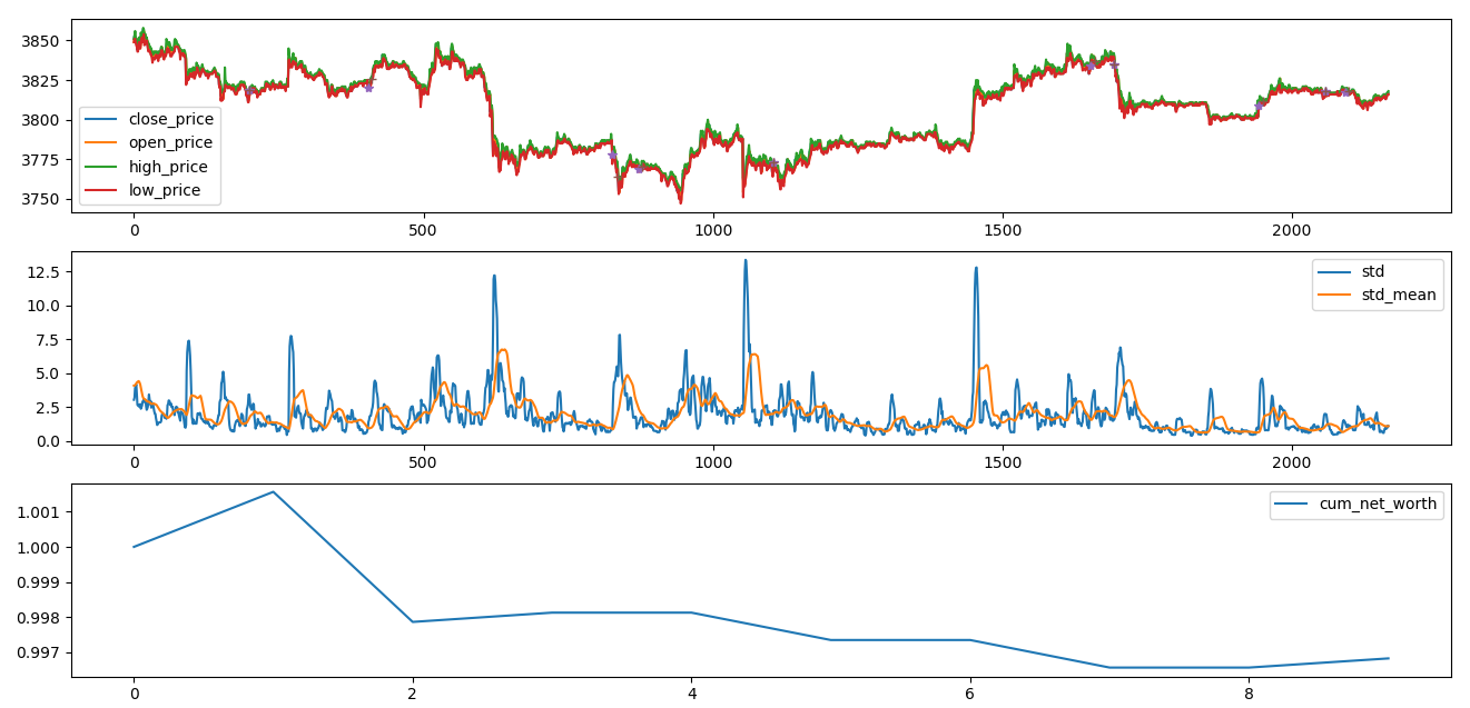
# #画出净值走势图
fig=plt.figure()
ax1=fig.add_subplot(3,1,1)
ag_close_price,=plt.plot(new_data['close_price'].values,label='close_price')
ag_open_price,=plt.plot(new_data['open_price'].values,label='open_price')
ag_high_price,=plt.plot(new_data['high_price'].values,label='high_price')
ag_low_price,=plt.plot(new_data['low_price'].values,label='low_price')
plt.legend([ag_close_price,ag_open_price,ag_high_price,ag_low_price],['close_price','open_price','high_price','low_price'])
ag_close_price_mark_enter=new_data.iloc[:,0].values.tolist()
ag_close_price_mark_leave=new_data.iloc[:,0].values.tolist()
# print(type(spread),type(spread_mark))
for i in range(0,T):
if mark_enter[i]==0:
ag_close_price_mark_enter[i]=nan
plt.plot(ag_close_price_mark_enter,'*')
for i in range(0,T):
if mark_leave[i]==0:
ag_close_price_mark_leave[i]=nan
plt.plot(ag_close_price_mark_leave,'+')
ax2=fig.add_subplot(3,1,2)
ag_std,=plt.plot(std,label='std')
ag_std_mean,=plt.plot(std_mean,label='std_mean')
plt.legend([ag_std,ag_std_mean],['std','std_mean'])
ax3=fig.add_subplot(3,1,3)
cum_net_worth,=plt.plot(df_cum,label='cum_net_worth')
plt.legend([cum_net_worth],['cum_net_worth'])
plt.show()
pdb.set_trace()
下面为运行结果图: