何为梯度下降,直白点就是,链式求导法则,不断更新变量值。
这里讲解的代码为李宏毅老师机器学习课程中 class 4 回归展示 中的代码demo
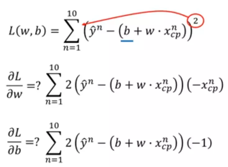
Loss函数
python代码如下
import numpy as np
import matplotlib.pyplot as plt

# y_data = b + w * x_data
x_data = [338., 333., 328., 207., 226., 25., 179., 60., 208., 606.]   # 10 个数
y_data = [640., 633., 619., 393., 428., 27., 193., 66., 226., 1591.]  # 10 个数

x = np.arange(-200, -100, 1)     # bias
y = np.arange(-5, 5, 0.1)        # weight
z = np.zeros((len(x), len(y)))   # zeros函数表示输出的数组为 100行 100列

#X, Y = np.meshgrid(x, y)  个人感觉这句话没用。。。

for i in range(len(x)):
    for j in range(len(y)):
        b = x[i]
        w = y[j]
        z[j][i] = 0
        for n in range(len(x_data)):
            # z[j][i]为 b=x[i] 及 w=y[j] 时,对应的 Loss Function 的大小
            z[j][i] = z[j][i] + (y_data[n] - b - w * x_data[n]) ** 2
        z[j][i] = z[j][i] / len(x_data)    # 求 loss function 均值

# y_data = b + w * x_data
b = -120              # initial b
w = -4                # initial w
lr = 0.0000001          # learning rate
iteration = 100000    # 迭代运行次数

# store initial values for plotting
b_history = [b]
w_history = [w]

# iterations
for i in range(iteration):      # 在 100000 次迭代下,看最后结果
    b_grad = 0.0                # 对 b_grad 重新赋值为0
    w_grad = 0.0                # 对 w_grad 重新赋值为0
    for n in range(len(x_data)):
        # 此处应该注意的是,求导的是Loss函数,因此对应的变量是w、b,是看w、b在各自的轴上的移动
        b_grad = b_grad + 2.0 * (y_data[n] - b - w * x_data[n]) * ( - 1.0)
        w_grad = w_grad + 2.0 * (y_data[n] - b - w * x_data[n]) * ( - x_data[n])

    # update parameters
    b = b - lr * b_grad
    w = w - lr * w_grad

    # store parameters for plotting
    b_history.append(b)
    w_history.append(w)

# plot the figure
plt.contourf(x, y, z, 50, alpha = 0.5, cmap = plt.get_cmap('jet'))
plt.plot([-188.4], [2.67], 'x', ms = 12, markeredgewidth = 3, color = 'orange')
plt.plot(b_history, w_history, 'o-', ms = 3, lw = 1.5, color = 'black')
plt.xlim(-200, -100)
plt.ylim(-5, 5)
plt.xlabel(r'$b$', fontsize=16)
plt.ylabel(r'$w$', fontsize=16)
plt.show()
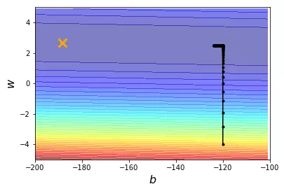
当learning rate 即 lr = 0.0000001时
当learning rate 即 lr = 0.000001时

learning rate 即 lr = 0.00001时

可以看到效果不是很好 所以改变learning rate
import numpy as np
import matplotlib.pyplot as plt

# y_data = b + w * x_data
x_data = [338., 333., 328., 207., 226., 25., 179., 60., 208., 606.]  # 10 个数
y_data = [640., 633., 619., 393., 428., 27., 193., 66., 226., 1591.]  # 10 个数

x = np.arange(-200, -100, 1)  # bias
y = np.arange(-5, 5, 0.1)  # weight
z = np.zeros((len(x), len(y)))  # zeros函数表示输出的数组为 100 行 100 列

# X, Y = np.meshgrid(x, y)

for i in range(len(x)):
    for j in range(len(y)):
        b = x[i]
        w = y[j]
        z[j][i] = 0
        for n in range(len(x_data)):
            # z[j][i]为 b=x[i] 及 w=y[j] 时,对应的 Loss Function 的大小
            z[j][i] = z[j][i] + (y_data[n] - b - w * x_data[n]) ** 2
        z[j][i] = z[j][i] / len(x_data)  # 求 loss function 均值

# ydata = b + w * xdata
b = -120  # initial b
w = -4  # initial w
lr = 1  # learning rate
iteration = 100000  # 迭代运行次数

# store initial values for plotting
b_history = [b]
w_history = [w]

# 个性化 w 和 b 的 learning rate
lr_b = 0
lr_w = 0

# iterations
for i in range(iteration):  # 在 100000 次迭代下,看最后结果
    b_grad = 0.0  # 对 b_grad 重新赋值为0
    w_grad = 0.0  # 对 w_grad 重新赋值为0
    for n in range(len(x_data)):
        # 此处应该注意的是,求导的是L函数,因此对应的变量是w、b,是看w、b在各自的轴上的移动
        b_grad = b_grad + 2.0 * (y_data[n] - b - w * x_data[n]) * (- 1.0)
        w_grad = w_grad + 2.0 * (y_data[n] - b - w * x_data[n]) * (- x_data[n])

    lr_b = lr_b + b_grad ** 2
    lr_w = lr_w + w_grad ** 2

    # update parameters
    b = b - lr / np.sqrt(lr_b) * b_grad
    w = w - lr / np.sqrt(lr_w) * w_grad

    # store parameters for plotting
    b_history.append(b)
    w_history.append(w)

# plot the figure
plt.contourf(x, y, z, 50, alpha=0.5, cmap=plt.get_cmap('jet'))
plt.plot([-188.4], [2.67], 'x', ms=12, markeredgewidth=3, color='orange')
plt.plot(b_history, w_history, 'o-', ms=3, lw=1.5, color='black')
plt.xlim(-200, -100)
plt.ylim(-5, 5)
plt.xlabel(r'$b$', fontsize=16)
plt.ylabel(r'$w$', fontsize=16)
plt.show()
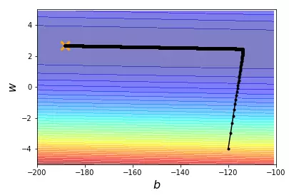
结果展示
一些说明:
np.array np.asarray的区别
array和asarry都可以将结构数据转换为ndarray类型
但是主要的区别在于当数据源是ndarray时,array仍会copy出一个副本,占用新的内存,但asarray不会。
np.meshgrid的作用
生成网格点坐标矩阵